<?xml version="1.0" encoding="utf-8"?><feed xmlns="http://www.w3.org/2005/Atom" xml:lang="en-US"><generator uri="https://jekyllrb.com/" version="4.4.1">Jekyll</generator><link href="https://www.ryancompton.net/feed.xml" rel="self" type="application/atom+xml" /><link href="https://www.ryancompton.net/" rel="alternate" type="text/html" hreflang="en-US" /><updated>2026-05-13T02:36:13+00:00</updated><id>https://www.ryancompton.net/feed.xml</id><title type="html">Ryan Compton</title><subtitle>Ryan Compton personal blog.</subtitle><author><name>Ryan Compton</name><email>ryan@ryancompton.net</email></author><entry><title type="html">Flying magnets! How do they work?!</title><link href="https://www.ryancompton.net/2025/08/16/flying-magnet-korg-monologue.html" rel="alternate" type="text/html" title="Flying magnets! How do they work?!" /><published>2025-08-16T00:00:00+00:00</published><updated>2025-08-16T00:00:00+00:00</updated><id>https://www.ryancompton.net/2025/08/16/flying-magnet-korg-monologue</id><content type="html" xml:base="https://www.ryancompton.net/2025/08/16/flying-magnet-korg-monologue.html"><![CDATA[<p>Years ago, during the start of covid, I wanted to replicate the <a href="https://mekonik.wordpress.com/2009/03/02/my-first-arduino-project/">Arduino magnetic levitation system</a> I saw my colleague build back in 2009. I know almost nothing about electrical engineering or control systems and when I tried this in 2020 I wasn’t even close to making it work. But now armed with LLMs, a 3D printer, and a willingness to buy whatever was needed from AliExpress I made the magnet fly! I even attached it to my Korg Monologue to sonify the control loop. Here’s proof:</p>

<iframe width="560" height="315" src="https://www.youtube.com/embed/qTpemqAp6Q0" frameborder="0" allow="accelerometer; autoplay; clipboard-write; encrypted-media; gyroscope; picture-in-picture" allowfullscreen=""></iframe>

<!--more-->

<h2 id="background">Background</h2>

<p>You can’t balance two permanent magnets in the just the right way to get levitation. It’s impossible. <a href="https://en.wikipedia.org/wiki/Earnshaw%27s_theorem#:~:text=Earnshaw's%20theorem%20states%20that%20a,mathematician%20Samuel%20Earnshaw%20in%201842.">Earnshaw’s theorem</a> proves it. The hack to make maglev possible is to use one permanent magnet and one dynamic magnet which is controled by some system. The common approach is to use an electromagnet and a <a href="https://en.wikipedia.org/wiki/Proportional%E2%80%93integral%E2%80%93derivative_controller">PID loop</a> (which is what I ended up doing) but it’s also possible to use <a href="https://en.wikipedia.org/wiki/Spin-stabilized_magnetic_levitation">gyroscopic stability</a>, superconductors, diamagnets, or <a href="https://en.wikipedia.org/wiki/Strong_focusing">strong focusing</a>.</p>

<p>There are plenty of videos online with people floating their magnets while calmly talking about how they set up the device and everything worked no problem, #diy #simpleproject #stemlearningforkids. These are all lies. Despite what you may be led to believe, getting that magnet to fly is horrifically difficult. It took me weeks (months?) of trial and error to get it right. I even saw some videos where they built up the whole system and started controlling the magnet but only at the very end do they reveal that they never got their magnet to fly. Never see that kind of thing of YouTube.</p>

<h2 id="materials">Materials</h2>

<p>Here’s what we need:</p>

<ul>
  <li>A permanent magnet</li>
  <li>An electromaget</li>
  <li>A power supply for the electromagnet</li>
  <li>A sensor to measure the distance between the magnets</li>
  <li>A computer to control the distance the distance between the magnets</li>
  <li>A platform to put everything on</li>
</ul>

<h3 id="the-permanent-magnet">The permanent magnet.</h3>

<p>This one is easy. I bought a pack of neodynium magnets years ago to upgrade our collection of things stuck to the refridgerator and used a couple of those. Here’s a closeup of the permanent magnet. I stuck some cardboard onto it so soften the impact when it collides with the sensors.</p>

<p><img src="https://www.ryancompton.net/assets/pix/perm_magnet.jpg" alt="perm_magnet" /></p>

<h3 id="the-electromagnet">The electromagnet.</h3>

<p>There are a lot more options here. I initially tried the cheapest electromagnet I could get on Amazon and it never felt like it had enough juice to get anything flying. Maybe if I tuned the system perfectly and kept the levitating magnet very close it could have worked but I wasn’t having any luck and started experimenting with larger magnets.</p>

<h4 id="option-1--large-iron-core-magnet">Option #1 – Large iron core magnet</h4>

<p>The most powerful magnet I tried had an iron core and was measured at 116.3mH. This could pull anything but I was having trouble tuning the PID loop with it.</p>

<p><img src="https://www.ryancompton.net/assets/pix/big_iron_core.jpg" alt="big_iron_core" /></p>

<p>Perhaps its switching speed is too slow? To measure switching spped I wrote a script on my raspberry pi to flip the magnet on/off in one thread while a seperate thread records readings from a Hall Effect sensor very close to the magnet. Here are the results for the big magnet:</p>

<p><img src="https://www.ryancompton.net/assets/pix/big_steel_magnet_switching_times.png" alt="big_steel_magnet_switching_times.png" /></p>

<h4 id="option-2--homemade-magnet">Option #2 – Homemade magnet</h4>

<p>I suspected I could build a magnet with faster switching times that’s still quite powerful by wrapping <a href="https://en.wikipedia.org/wiki/Magnet_wire">magnet wire</a> around a ferrite core. It took a long time wrapping that wire and I only got 26mH out of it.</p>

<p><img src="https://www.ryancompton.net/assets/pix/artisanal_magnet.JPEG" alt="artisanal_magnet" /></p>

<p>This magnet would get very hot if I played with it for too long. The 3D printed case would soften up and start to melt. There was loud coil whine. The switching speed was very fast but the magnetic field was complicated.</p>

<p><img src="https://www.ryancompton.net/assets/pix/homemade_magnet_switching.png" alt="homemade_magnet_switching" /></p>

<h4 id="option-3-selected--air-core-solenoid">Option #3 (selected) – Air core solenoid</h4>

<p>Electromagnets are useful for controlling water flow. There’s a solenoid valve in my espresso machine. I bought a reasonably large solenoid on Alibaba.</p>

<p><img src="https://www.ryancompton.net/assets/pix/alimag.JPEG" alt="aircore_magnet_ad" /></p>

<p>It only measured 9.72mH but that was plenty for my experiment.</p>

<p><img src="https://www.ryancompton.net/assets/pix/aircore_magnet.jpg" alt="aircore_magnet" /></p>

<p>The air core magnet switches very fast:</p>

<p><img src="https://www.ryancompton.net/assets/pix/alibaba_big_solenoid_air_gap_switch.png" alt="air_core_magnet_switching" /></p>

<h3 id="the-power-supply">The Power Supply</h3>

<p>The raspberry pi only outputs logic voltage of 3.3V. I need more to power these big magnets. The way to solve this is for the pi to switch a MOSFET which in turn drives current to the magnet. I tried a 9V battery at first. That did not work. 9V batteries have very high internal resistance and can not supply much current. I tried a little RC car power supply also without much luck.</p>

<p>The eventual champion of the power supply bracket was the DP100. I really like this thing and have been using it for all kinds of stuff since buying it for this project.</p>

<p><img src="https://www.ryancompton.net/assets/pix/dp100.jpg" alt="dp100" /></p>

<h3 id="sensors">Sensors</h3>

<p>To measure the distance between the permanent magnet and the electromagnet I used a Hall Effect sensor placed <strong>underneath</strong> the permanent magnet. Placing the Hall Effect sensor far from the electromagnet greatly simplifes this project because, since magnetic field is inverse to the square of the distance, it means that the sensor will primarily measure the field from the permanent magnet rather than a combined field that includes both magnets. Here it is under the magnet:</p>

<p><img src="https://www.ryancompton.net/assets/pix/hallsensor.jpg" alt="hallsensor" /></p>]]></content><author><name>Ryan Compton</name><email>ryan@ryancompton.net</email></author><category term="magnets" /><category term="audio" /><summary type="html"><![CDATA[Years ago, during the start of covid, I wanted to replicate the Arduino magnetic levitation system I saw my colleague build back in 2009. I know almost nothing about electrical engineering or control systems and when I tried this in 2020 I wasn’t even close to making it work. But now armed with LLMs, a 3D printer, and a willingness to buy whatever was needed from AliExpress I made the magnet fly! I even attached it to my Korg Monologue to sonify the control loop. Here’s proof:]]></summary></entry><entry><title type="html">Surf Bikes!</title><link href="https://www.ryancompton.net/2024/03/03/surfbikes.html" rel="alternate" type="text/html" title="Surf Bikes!" /><published>2024-03-03T00:00:00+00:00</published><updated>2024-03-03T00:00:00+00:00</updated><id>https://www.ryancompton.net/2024/03/03/surfbikes</id><content type="html" xml:base="https://www.ryancompton.net/2024/03/03/surfbikes.html"><![CDATA[<p>On a few occasions I’ve been fortunate enough to live within biking distance of a surf break. One of my favorite activities to do in this situation is outfit a bicycle with a surfboard rack and use it for transportation to the beach.</p>

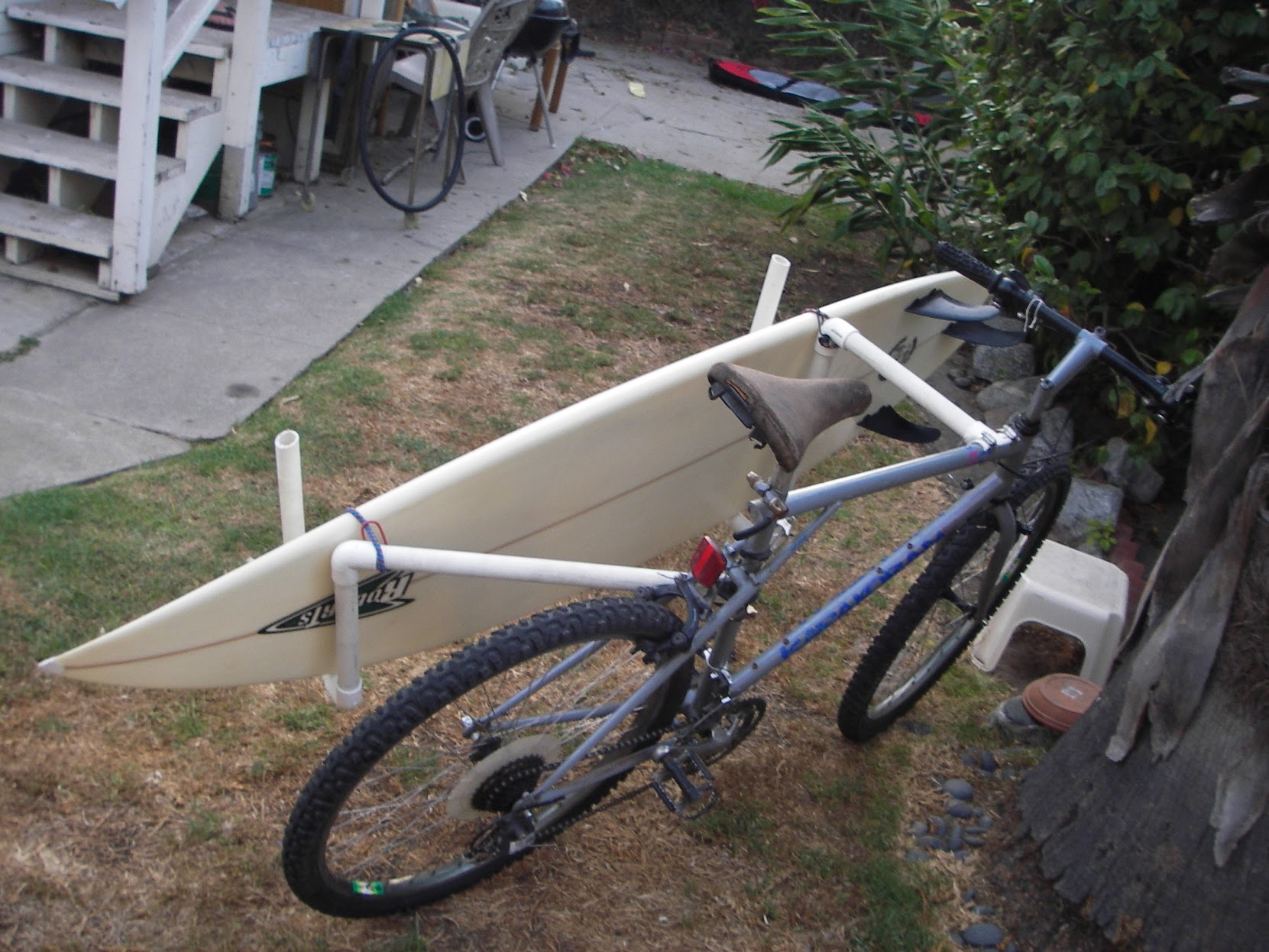
<p>Here are the bikes. PVC construction inspired by <a href="http://www.rodndtube.com/surf/info/surf_racks/BicycleSurfboardRack.shtml">http://www.rodndtube.com/surf/info/surf_racks/BicycleSurfboardRack.shtml</a>.</p>

<h2 id="gt-karakoram--2007">GT Karakoram – 2007</h2>

<p><img src="https://www.ryancompton.net/assets/pix/grey_bike.jpeg" alt="grey_bike" /></p>

<p>I got this bicycle for free when I purchased my first mountain bike from someone on Craigslist in Glendale in late 2006. I took both bicycles back to Westwood via bus where I was promptly stopped and questioned by the police as to why I had two bikes with me on the bus. Neither showed up as reported missing so they let me out. The next year I moved to Santa Monica near Wilshire and 17th Street and built this rack so I could ride to Venice Beach to surf in the morning. The ride was long and the waves were bad but I enjoyed every minute of it.</p>

<p>In 2008 I moved too far from the coast for this to be practical so I donated the bicycle to <a href="https://bikerowave.org/">Bikerowave</a> and didn’t put another one together for ~10 years.</p>

<!--more-->

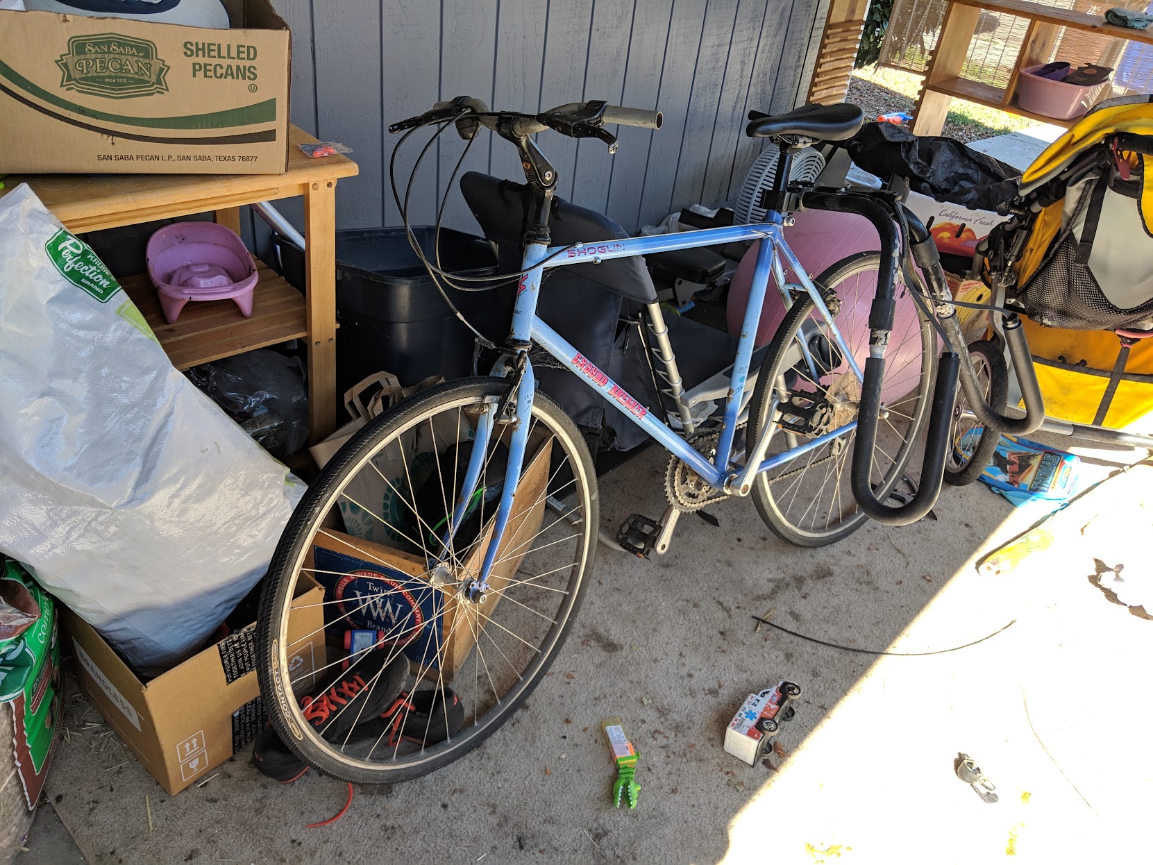
<h2 id="shogun-unknown-model--2017">Shogun (unknown model) – 2017</h2>

<p><img src="https://www.ryancompton.net/assets/pix/shogun_bike.jpeg" alt="shogun_bike" /></p>

<p>When I started working at Google we moved to Santa Cruz and I rode the corp bus into Mountain View every morning. But if I got up early enough I could sneak in a quick session, usually at Steamer Lane, before work via bicycle. This bike, an unknown model built by Shogun, was discarded by one of my neighbors. I fixed it up and slapped an off-the-shelf surfboard rack on it so I could get right up to the cliff and lock it on the fence overlooking the ocean. It lasted almost a year until someone stole it from the carport while I was in the backyard putting my board in the shed.</p>

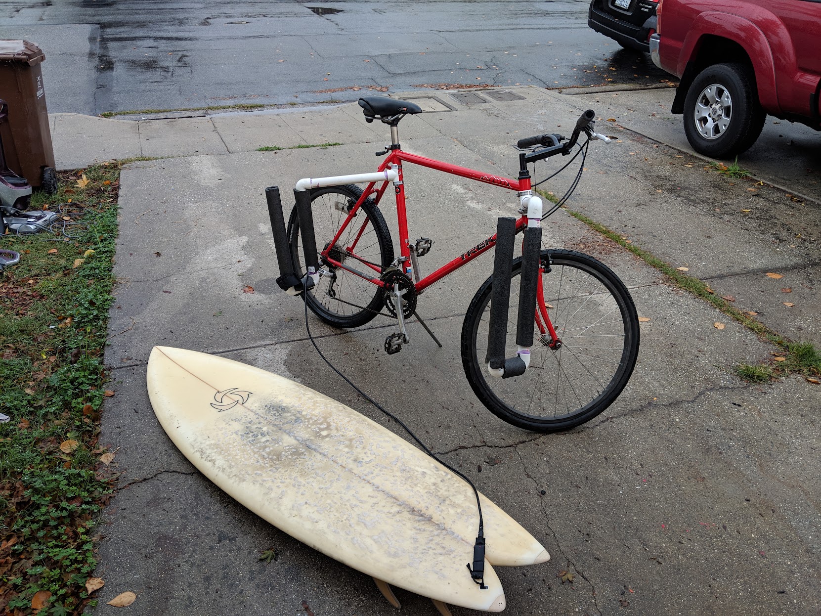
<h2 id="trek-800--2018">Trek 800 – 2018</h2>

<p><img src="https://www.ryancompton.net/assets/pix/red_bike.jpeg" alt="red_bike" /></p>

<p>After the Shogun was stolen I picked up this from someone on Craigslist and rode it home in the rain. I opted to build another PVC rack this time as I was unimpressed with the one I bought for the Shogun. When we moved away from Santa Cruz I gave it away.</p>

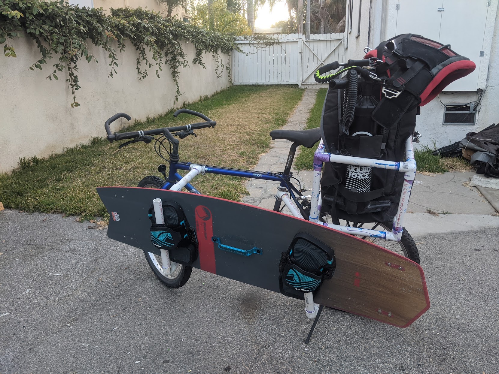
<h2 id="univega-alpina-sport--2020">Univega Alpina Sport – 2020</h2>

<p><img src="https://www.ryancompton.net/assets/pix/kite_bike.jpeg" alt="kite_bike" /></p>

<p>When we moved to Long Beach I effectively gave up on surfing as <a href="https://www.latimes.com/california/story/2019-12-18/long-beach-breakwater-wont-be-removed">the breakwater blocks all the waves and will never go away</a>. Luckily, Belmont Shore is a great place to kiteboard and kite gear is pretty compact. I fit my rig onto the same PVC rack used earlier with some extra stuff on the back. It works, but the huge downside to this is that riding around when the wind is 20kts is not a great activity.</p>

<h2 id="et-cycles-720--2023">ET Cycles 720 – 2023</h2>

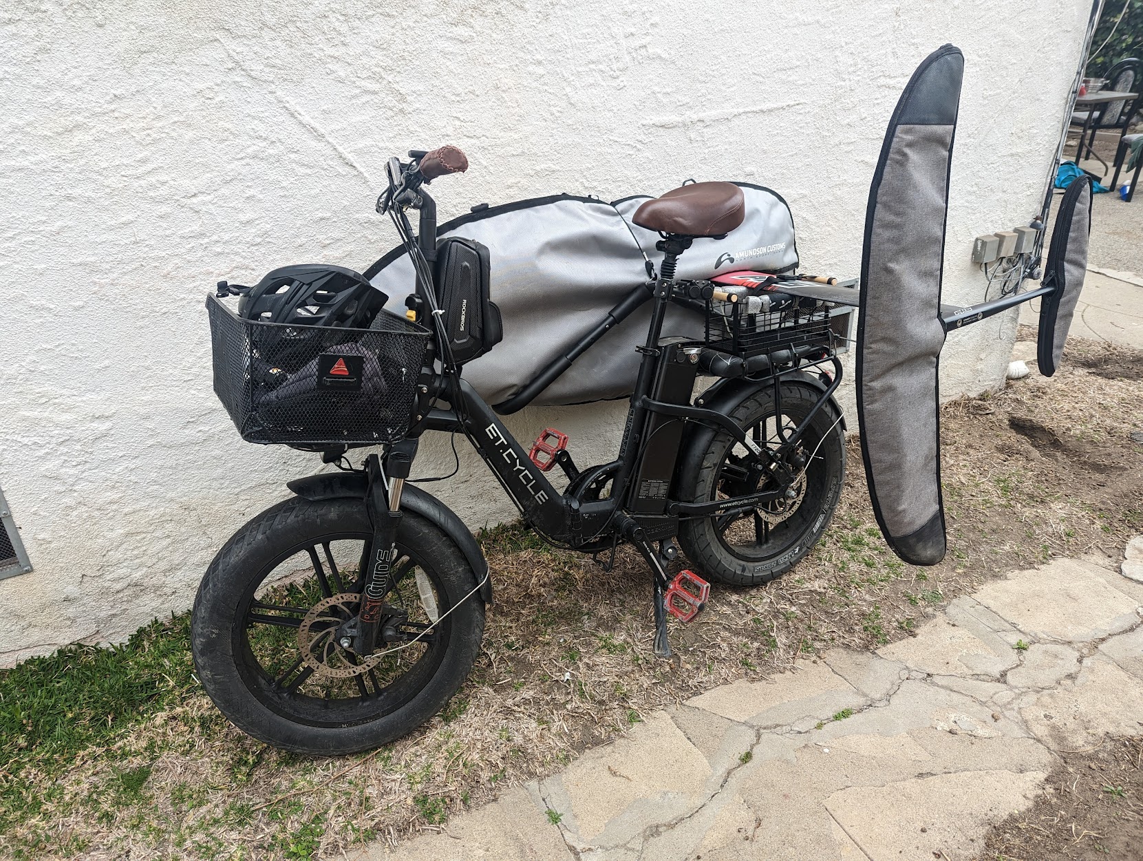
<p><img src="https://www.ryancompton.net/assets/pix/foil_bike.jpeg" alt="foil_bike" /></p>

<p>Kiteboarding is fun, but it’s quite different from surfing as you’re getting pulled by the wind instead of the waves. I was never able to shake this and eventually found myself back in the waves at Seal Beach. Seal Beach is arguably the best foil wave on the West Coast and I couldn’t be happier about the new sport. It’s a few miles from the building we live in so I was driving there. One night our catalytic converter was stolen and the wait for a replacement was 6+ months. This is how I discovered e-bikes and <strong>they are amazing</strong>, like riding downhill the whole way. I used an off the shelf rack for this build because the foil gets in the way of the PVC rack I’m familiar with. There’s also a box on the back that holds the mast high to prevent the wing from dragging during a turn.</p>

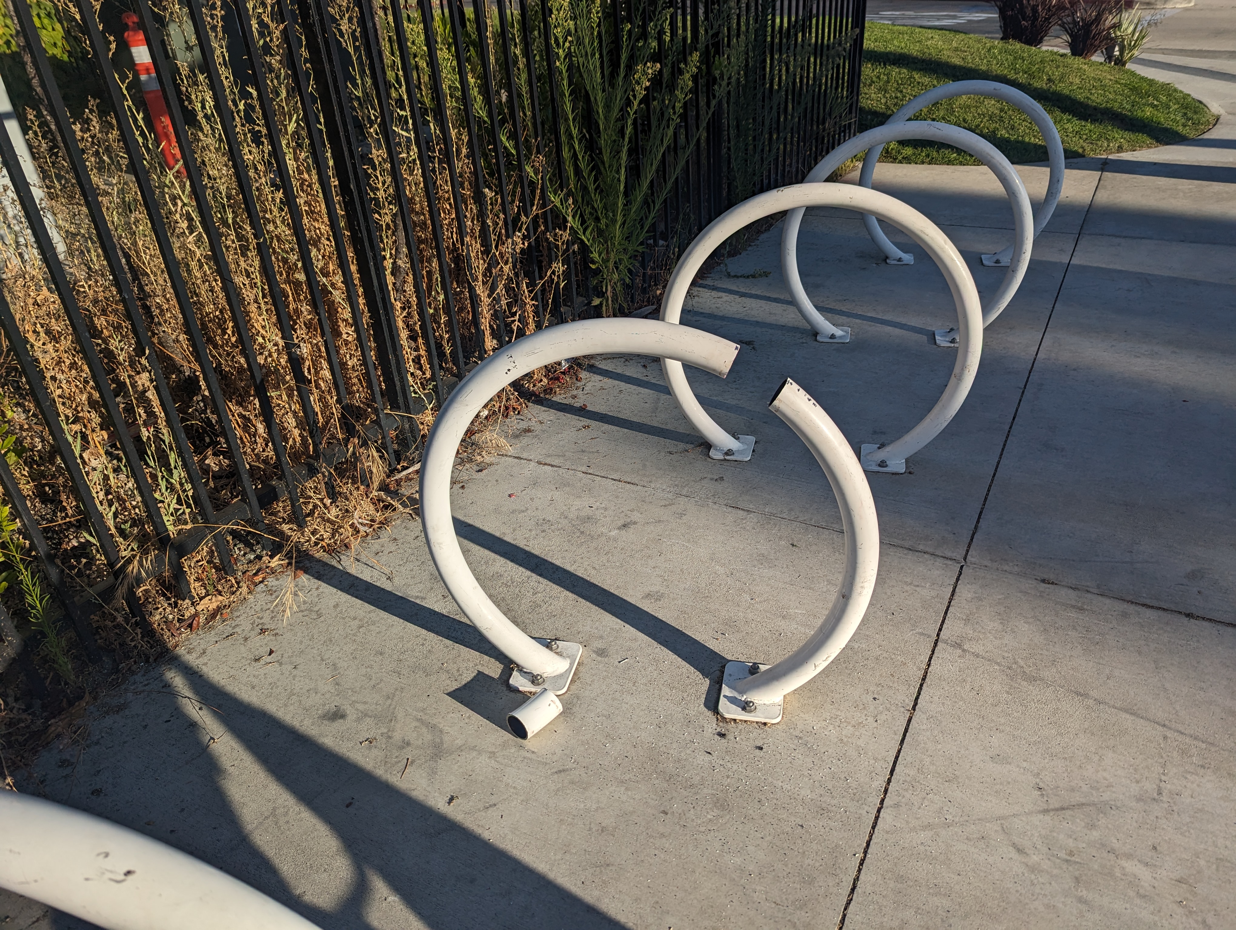
<p>when I was at KDD 2023 I locked this up outside the Long Beach Convention Center for a day with a powerful Kryptonite lock. But the city apparently doesn’t install strong bike racks and my e-bike was taken.</p>

<p><img src="https://www.ryancompton.net/assets/pix/PXL_20230808_012407085.MP.jpg" alt="lbc_rack" /></p>]]></content><author><name>Ryan Compton</name><email>ryan@ryancompton.net</email></author><category term="surfing" /><summary type="html"><![CDATA[On a few occasions I’ve been fortunate enough to live within biking distance of a surf break. One of my favorite activities to do in this situation is outfit a bicycle with a surfboard rack and use it for transportation to the beach. Here are the bikes. PVC construction inspired by http://www.rodndtube.com/surf/info/surf_racks/BicycleSurfboardRack.shtml. GT Karakoram – 2007 I got this bicycle for free when I purchased my first mountain bike from someone on Craigslist in Glendale in late 2006. I took both bicycles back to Westwood via bus where I was promptly stopped and questioned by the police as to why I had two bikes with me on the bus. Neither showed up as reported missing so they let me out. The next year I moved to Santa Monica near Wilshire and 17th Street and built this rack so I could ride to Venice Beach to surf in the morning. The ride was long and the waves were bad but I enjoyed every minute of it. In 2008 I moved too far from the coast for this to be practical so I donated the bicycle to Bikerowave and didn’t put another one together for ~10 years.]]></summary></entry><entry><title type="html">Enable HTTPS for S3, Cloudfront, Namecheap</title><link href="https://www.ryancompton.net/2023/01/11/https.html" rel="alternate" type="text/html" title="Enable HTTPS for S3, Cloudfront, Namecheap" /><published>2023-01-11T00:00:00+00:00</published><updated>2023-01-11T00:00:00+00:00</updated><id>https://www.ryancompton.net/2023/01/11/https</id><content type="html" xml:base="https://www.ryancompton.net/2023/01/11/https.html"><![CDATA[<p>I finally got around to enabling https here. Some notes:</p>

<ol>
  <li>
    <p>Namecheap sells ssl certs via PositiveSSL/Comodo. I thought this would be easiest but they don’t really work with AWS.</p>

    <ul>
      <li>I’ll never get that $7 back</li>
      <li>It’s more work to import a 3rd party certificate vs. creating one on AWS</li>
      <li>After importing the 3rd party certificate (which has to happen in N. Virgina) AWS still claims that it’s not from a trusted source</li>
      <li><a href="https://stackoverflow.com/questions/51198472/cname-entry-not-working-on-namecheap-using-amazon-certificate-manager">Other CNAME gotchas</a></li>
    </ul>
  </li>
  <li>
    <p>Amazon Certificate Manager allows one to create the certificate from AWS for free</p>

    <ul>
      <li>They’ll auto generate the Route 53 CNAME rules for you</li>
      <li>Still the same weird thing about how you need to do this in N. Virginia even if the rest of you site is elsewhere</li>
    </ul>
  </li>
  <li>
    <p>You need to add an “alias” rule to point your custom domain at Cloudfront.</p>
  </li>
</ol>

<p>I found <a href="https://davelms.medium.com/using-a-custom-domain-in-cloudfront-with-an-ssl-certificate-and-route-53-253a72f51056">this blog</a> helpful</p>]]></content><author><name>Ryan Compton</name><email>ryan@ryancompton.net</email></author><category term="coding" /><summary type="html"><![CDATA[I finally got around to enabling https here. Some notes: Namecheap sells ssl certs via PositiveSSL/Comodo. I thought this would be easiest but they don’t really work with AWS. I’ll never get that $7 back It’s more work to import a 3rd party certificate vs. creating one on AWS After importing the 3rd party certificate (which has to happen in N. Virgina) AWS still claims that it’s not from a trusted source Other CNAME gotchas Amazon Certificate Manager allows one to create the certificate from AWS for free They’ll auto generate the Route 53 CNAME rules for you Still the same weird thing about how you need to do this in N. Virginia even if the rest of you site is elsewhere You need to add an “alias” rule to point your custom domain at Cloudfront. I found this blog helpful]]></summary></entry><entry><title type="html">Migrating off s3_website.yml</title><link href="https://www.ryancompton.net/2023/01/10/s3_website.html" rel="alternate" type="text/html" title="Migrating off s3_website.yml" /><published>2023-01-10T00:00:00+00:00</published><updated>2023-01-10T00:00:00+00:00</updated><id>https://www.ryancompton.net/2023/01/10/s3_website</id><content type="html" xml:base="https://www.ryancompton.net/2023/01/10/s3_website.html"><![CDATA[<p>First post in 5+ years! I used to use <a href="https://github.com/laurilehmijoki/s3_website">s3_website</a> to publish this blog. Turns out that project has been deprecated with nothing to replace it. Oh well.</p>

<p><a href="https://pagertree.com/blog/jekyll-site-to-aws-s3-using-github-actions">Following this</a> I’ve managed to setup Github Actions to build/deploy the blog. A few small changes:</p>

<!--more-->

<ul>
  <li>Github stuff tends to default to <code class="language-plaintext highlighter-rouge">main</code> now but this repository is old and uses <code class="language-plaintext highlighter-rouge">master</code></li>
  <li>the [email protected] stuff in their blog post wasn’t working for me</li>
</ul>

<p>Here’s the deploy script I’m using to publish this post:</p>

<figure class="highlight"><pre><code class="language-yaml" data-lang="yaml"><span class="na">name</span><span class="pi">:</span> <span class="s">Jekyll build and S3 deploy</span>

<span class="na">on</span><span class="pi">:</span>
  <span class="na">push</span><span class="pi">:</span>
    <span class="na">branches</span><span class="pi">:</span> <span class="pi">[</span> <span class="nv">master</span> <span class="pi">]</span>

  <span class="c1"># Allows you to run this workflow manually from the Actions tab</span>
  <span class="na">workflow_dispatch</span><span class="pi">:</span>


<span class="na">env</span><span class="pi">:</span>
  <span class="na">AWS_ACCESS_KEY_ID</span><span class="pi">:</span> <span class="s">${{ secrets.AWS_ACCESS_KEY_ID }}</span>
  <span class="na">AWS_SECRET_ACCESS_KEY</span><span class="pi">:</span> <span class="s">${{ secrets.AWS_SECRET_ACCESS_KEY }}</span>
  <span class="na">AWS_DEFAULT_REGION</span><span class="pi">:</span> <span class="s1">'</span><span class="s">us-west-2'</span>


<span class="na">jobs</span><span class="pi">:</span>
  <span class="na">build_and_deploy</span><span class="pi">:</span>
    <span class="na">runs-on</span><span class="pi">:</span> <span class="s">ubuntu-latest</span>
    <span class="na">steps</span><span class="pi">:</span>
      <span class="pi">-</span> <span class="na">uses</span><span class="pi">:</span> <span class="s">actions/checkout@v3</span>
      
      <span class="pi">-</span> <span class="na">name</span><span class="pi">:</span> <span class="s">Set up Ruby</span>
        <span class="na">uses</span><span class="pi">:</span> <span class="s">ruby/setup-ruby@359bebbc29cbe6c87da6bc9ea3bc930432750108</span>
        <span class="na">with</span><span class="pi">:</span>
          <span class="na">ruby-version</span><span class="pi">:</span> <span class="s1">'</span><span class="s">3.1'</span>

      <span class="pi">-</span> <span class="na">name</span><span class="pi">:</span> <span class="s">Install dependencies</span>
        <span class="na">run</span><span class="pi">:</span> <span class="s">bundle install</span>

      <span class="pi">-</span> <span class="na">name</span><span class="pi">:</span> <span class="s2">"</span><span class="s">Build</span><span class="nv"> </span><span class="s">Site"</span>
        <span class="na">run</span><span class="pi">:</span> <span class="s">bundle exec jekyll build</span>
        <span class="na">env</span><span class="pi">:</span>
          <span class="na">JEKYLL_ENV</span><span class="pi">:</span> <span class="s">production</span>

      <span class="pi">-</span> <span class="na">name</span><span class="pi">:</span> <span class="s2">"</span><span class="s">Deploy</span><span class="nv"> </span><span class="s">to</span><span class="nv"> </span><span class="s">AWS</span><span class="nv"> </span><span class="s">S3"</span>
        <span class="na">run</span><span class="pi">:</span> <span class="s">aws s3 sync ./_site/ s3://${{ secrets.AWS_S3_BUCKET_NAME }} --acl public-read --delete --cache-control max-age=604800</span>

      <span class="pi">-</span> <span class="na">name</span><span class="pi">:</span> <span class="s2">"</span><span class="s">Create</span><span class="nv"> </span><span class="s">AWS</span><span class="nv"> </span><span class="s">Cloudfront</span><span class="nv"> </span><span class="s">Invalidation"</span>
        <span class="na">run</span><span class="pi">:</span> <span class="s">aws cloudfront create-invalidation --distribution-id ${{ secrets.AWS_CLOUDFRONT_DISTRIBUTION_ID }} --paths "/*"</span></code></pre></figure>]]></content><author><name>Ryan Compton</name><email>ryan@ryancompton.net</email></author><category term="coding" /><summary type="html"><![CDATA[First post in 5+ years! I used to use s3_website to publish this blog. Turns out that project has been deprecated with nothing to replace it. Oh well. Following this I’ve managed to setup Github Actions to build/deploy the blog. A few small changes:]]></summary></entry><entry><title type="html">One thousand captcha photos organized with a neural network</title><link href="https://www.ryancompton.net/2017/08/18/one-thousand-captcha-photos-organized-with-a-neural-network.html" rel="alternate" type="text/html" title="One thousand captcha photos organized with a neural network" /><published>2017-08-18T00:00:00+00:00</published><updated>2017-08-18T00:00:00+00:00</updated><id>https://www.ryancompton.net/2017/08/18/one-thousand-captcha-photos-organized-with-a-neural-network</id><content type="html" xml:base="https://www.ryancompton.net/2017/08/18/one-thousand-captcha-photos-organized-with-a-neural-network.html"><![CDATA[<p><em>Coauthored with Habib Talavati. Originally published on the Clarifai blog at <a href="https://blog.clarifai.com/one-thousand-captcha-photos-organized-with-a-neural-network-2/">https://blog.clarifai.com/one-thousand-captcha-photos-organized-with-a-neural-network-2/</a></em></p>

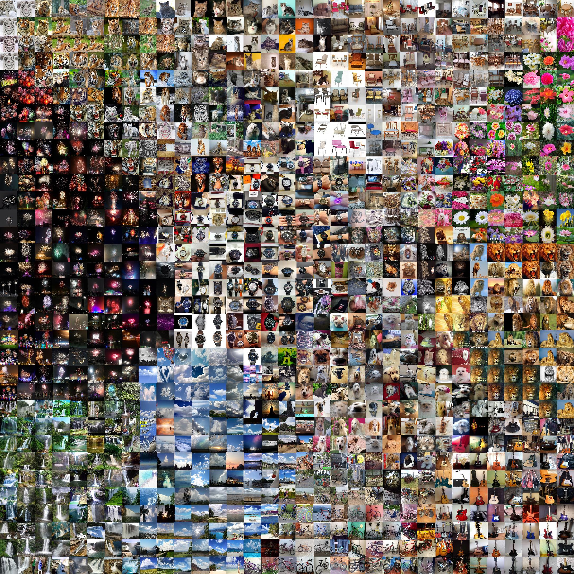
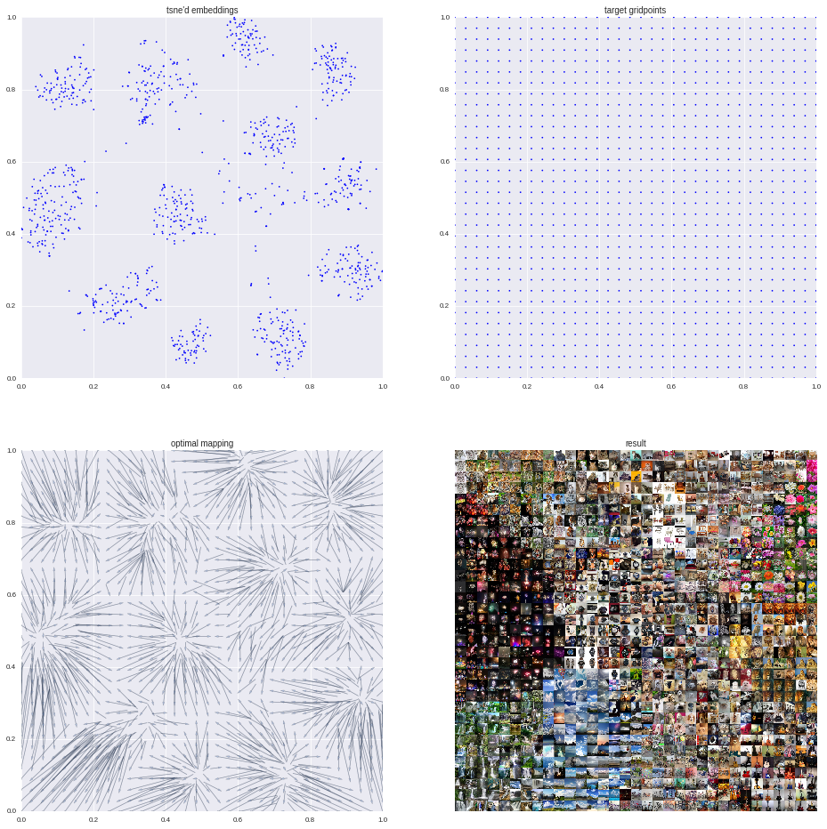
<p>The below image shows 1024 of the captcha photos used in “I’m not a human: Breaking the Google reCAPTCHA” by Sivakorn, Polakis, and Keromytis arranged on a 32x32 grid in such a way that visually-similar photos appear in close proximity to each other on the grid.</p>

<p><img src="https://www.ryancompton.net/assets/pix/gridz.jpg" alt="captcha bigimg" /></p>

<!--more-->

<h2 id="how-did-we-do-this">How did we do this?</h2>

<p>To get from the collection of captcha photos to the grid above we take three steps: embedding via a neural net, further dimension reduction via t-SNE, and finally snapping things to a grid by solving an assignment problem.</p>

<p>Images are naturally very high-dimensional objects, even a “small” 224x224 image requires 224<em>224</em>3=150,528 RGB values. When represented naively as huge vectors of pixels visually-similar images may have enormous vector distances between them. For example, a left/right flip will generate a visually-similar image but can easily lead to a situation where each pixel in the flipped version has an entirely different value from the original.</p>

<p><em>Remark:</em> Code for all of this is available here: <a href="https://github.com/Clarifai/public-notebooks/blob/master/gridded_tsne_blog_public.ipynb">https://github.com/Clarifai/public-notebooks/blob/master/gridded_tsne_blog_public.ipynb</a></p>

<p><img src="https://www.ryancompton.net/assets/pix/2x2captcha.png" alt="captcha_2x2" /></p>

<h3 id="step-1-reducing-from-150528-to-1024-dimensions-with-a-neural-net">Step 1: Reducing from 150528 to 1024 dimensions with a neural net</h3>

<p>Our photos begin as 224x224x3 arrays of RGB values. We pass each image through an existing pre-trained neural network, Clarifai’s <a href="https://developer.clarifai.com/models/general-embedding-image-recognition-model/bbb5f41425b8468d9b7a554ff10f8581">general embedding model</a> which provides us with the activations from one of the top layers of the net. Using the higher layers from a neural net provides us with representations of our images which are rich in semantic information - the vectors of visually similar images will be close to each other in the 1024-dimensional space.</p>

<h3 id="step-2-reducing-from-1024-to-2-dimensions-with-t-sne">Step 2: Reducing from 1024 to 2 dimensions with t-SNE</h3>

<p>In order to bring things down to a space where we can start plotting, we must reduce dimensions again. We have lots of options here. Some examples:</p>

<h4 id="inductive-methods-for-embedding-learning">Inductive methods for embedding learning</h4>

<p>Techniques such as the remarkably hard-to-Google <a href="http://yann.lecun.com/exdb/publis/pdf/hadsell-chopra-lecun-06.pdf">Dr. LIM</a> or Siamese Networks with triplet losses learn a function that can embed new images to fewer dimensions without any additional retraining. These techniques perform extremely well on benchmark datasets and are a great fit for online systems which must index previously-unseen images. For our application, we only need to get a fixed set of vectors reduced to 2D in one large, slow, step.</p>

<h4 id="transductive-methods-for-dimensionality-reduction">Transductive methods for dimensionality reduction</h4>

<p>Rather than learning a function which can new points to few dimensions we can attack our problem more directly by learning a mapping from the high-dimensional space to 2D which preserves distances in the high-dimensional space as much as possible. Several techniques are available: <a href="https://distill.pub/2016/misread-tsne/">t-SNE</a>, and <a href="https://github.com/lferry007/LargeVis">largeVis</a> to name a few. Other methods, such as PCA, are not optimized for distance preservation or visualization and tend to produce less interesting plots. t-SNE, even during convergence, can produce very interesting plots (cf. this demonstration by <a href="https://twitter.com/genekogan">@genekogan</a> <a href="https://vimeo.com/191187346">here</a> ).</p>

<p>We use t-SNE to map our 1024D vectors down to 2D and generate the first entry in the above grid. Recall that our high-dimensional space here are 1024D vector embeddings from a neural net, so proximal vectors show correspond to visually similar photos. Without the neural net t-SNE would be a poor choice as distances between the initial 224x224x3 vectors are uninteresting.</p>

<h3 id="step-3-snapping-to-a-grid-with-the-jonker-volgenant-algorithm">Step 3: Snapping to a grid with the Jonker-Volgenant algorithm</h3>

<p>One problem with t-SNE’d embeddings is that if we displayed the images directly over their corresponding 2D points we’d be left with swaths of empty white space and crowded regions where images overlap each other. We remedey this by building a 32x32 grid and moving the t-SNE’d points to the grid in such a way that total distance traveled is optimal.</p>

<p>It turns out that this operation can be incredibly sophisticated. There is an entire field of mathematics, <a href="https://en.wikipedia.org/wiki/Transportation_theory_(mathematics)">transportation theory</a>, concerned with solutions to problems in optimal transport under various circumstances. For example, if one’s goal is to minimize the sum of the squares of all distances traveled rather than simply the sum of the distances traveled (ie the l2 Monge-Kantorovitch mass transfer problem) an optimal mapping can be found by recasting the assignment problem as one in computational fluid dynamics and <a href="http://citeseerx.ist.psu.edu/viewdoc/download?doi=10.1.1.7.6791&amp;rep=rep1&amp;type=pdf">solving the corresponding PDEs</a>. <a href="https://en.wikipedia.org/wiki/C%C3%A9dric_Villani">Cedric Villani</a>, who won a Fields medal in 2010, wrote a great <a href="cedricvillani.org/wp-content/uploads/2012/08/preprint-1.pdf">book</a> on optimal transportation theory which is worth taking a look at when you get tired of corporate machine learning blogs.</p>

<p>In our setting, we just want the t-SNE’d points to snap to the grid in a way that makes this look visually appealing and be as simple as possible. Thus, we search for a mapping that minimizes the sum of the distances traveled via a <a href="https://en.wikipedia.org/wiki/Assignment_problem">linear assignment problem</a>. The textbook solution here is to use the <a href="https://en.wikipedia.org/wiki/Hungarian_algorithm">Hungarian algorithm</a>, however, this can be also be solved quite easily and much faster using <a href="https://blog.sourced.tech/post/lapjv/">Jonker-Volgenant</a> and <a href="https://github.com/src-d/lapjv">open source tools</a></p>

<h2 id="how-easy-can-we-make-this">How easy can we make this?</h2>

<p>Pretty easy. In addition to the notebook listed above, we’ve also set up an API endpoint that will generate an image similar to the one above for an existing Clarifai application. Here we assume you already have created an application by visiting https://developer.clarifai.com/account/applications and added your favorite images to it by calling the resource 
https://api.clarifai.com/v2/inputs. Then all you have to do is this:</p>

<h3 id="step-1-kick-off-an-asynchronous-gridded-t-sne-visualization">Step 1: Kick off an asynchronous gridded t-SNE visualization</h3>
<p>Since generating a visualization takes a while, we generate one asynchronously. We kick off a visualization by calling
<code class="language-plaintext highlighter-rouge">POST https://api.clarifai.com/v2/visualizations/</code></p>

<p>You should get a response like below informing us a “pending” visualization is scheduled to be computed</p>

<div class="language-plaintext highlighter-rouge"><div class="highlight"><pre class="highlight"><code>{
    "output": {
        "id": "ca69f34d53c742e1b4a1b71d7b4b4586",
        ...
    }
}
</code></pre></div></div>

<p>Note the id <code class="language-plaintext highlighter-rouge">ca69f34d53c742e1b4a1b71d7b4b4586</code>. We will use that id to get the visualization we just kicked off.</p>

<h3 id="step-2-check-to-see-if-the-visualization-is-done">Step 2: Check to see if the visualization is done</h3>
<p>Call <code class="language-plaintext highlighter-rouge">GET /v2/visualizations/ca69f34d53c742e1b4a1b71d7b4b4586</code>. The returned visualization will be “pending” for a while, but eventually, we should get a response like this:</p>

<div class="language-plaintext highlighter-rouge"><div class="highlight"><pre class="highlight"><code>{
    "output": {
        "data": {
            "image": {
                "url": "https://s3.amazonaws.com/clarifai-visualization/gridded-tsne/staging/your-visualization.jpg"
            }
        },
        ...
    }
}
</code></pre></div></div>

<p>At last, the <code class="language-plaintext highlighter-rouge">output.data.image.url</code> contains your gridded t-SNE visualization.</p>]]></content><author><name>Ryan Compton</name><email>ryan@ryancompton.net</email></author><category term="coding" /><category term="machine learning" /><summary type="html"><![CDATA[Coauthored with Habib Talavati. Originally published on the Clarifai blog at https://blog.clarifai.com/one-thousand-captcha-photos-organized-with-a-neural-network-2/ The below image shows 1024 of the captcha photos used in “I’m not a human: Breaking the Google reCAPTCHA” by Sivakorn, Polakis, and Keromytis arranged on a 32x32 grid in such a way that visually-similar photos appear in close proximity to each other on the grid.]]></summary></entry><entry><title type="html">My talk at the NYC Machine Learning meetup</title><link href="https://www.ryancompton.net/2016/12/06/my-talk-at-the-nyc-machine-learning-meetup.html" rel="alternate" type="text/html" title="My talk at the NYC Machine Learning meetup" /><published>2016-12-06T00:00:00+00:00</published><updated>2016-12-06T00:00:00+00:00</updated><id>https://www.ryancompton.net/2016/12/06/my-talk-at-the-nyc-machine-learning-meetup</id><content type="html" xml:base="https://www.ryancompton.net/2016/12/06/my-talk-at-the-nyc-machine-learning-meetup.html"><![CDATA[<p>Check out this video of my talk at the NYC Machine Learning meetup.</p>

<p>It’s based on this <a href="https://www.ryancompton.net/2016/04/19/what-convolutional-neural-networks-look-at-when-they-look-at-nudity/">blog post</a> and the deck is <a href="http://bit.ly/gdgny-dec2016-clarifai">here</a>.</p>

<div style="position: relative; padding-bottom: 56.25%; height: 0; overflow: hidden;">
  <iframe style="position: absolute; top: 0; left: 0; width: 100%; height: 100%;" src="https://www.youtube.com/embed/dWgXPKMvxDg" frameborder="0" allowfullscreen=""></iframe>
</div>]]></content><author><name>Ryan Compton</name><email>ryan@ryancompton.net</email></author><category term="machine learning" /><summary type="html"><![CDATA[Check out this video of my talk at the NYC Machine Learning meetup. It’s based on this blog post and the deck is here.]]></summary></entry><entry><title type="html">Upvotes over time by subreddit or: Why /r/The_Donald is always on the front page</title><link href="https://www.ryancompton.net/2016/08/07/upvotes-over-time-by-subreddit-or-why-the_donald-is-always-on-the-front-page-of-reddit.html" rel="alternate" type="text/html" title="Upvotes over time by subreddit or: Why /r/The_Donald is always on the front page" /><published>2016-08-07T00:00:00+00:00</published><updated>2016-08-07T00:00:00+00:00</updated><id>https://www.ryancompton.net/2016/08/07/upvotes-over-time-by-subreddit-or-why-the_donald-is-always-on-the-front-page-of-reddit</id><content type="html" xml:base="https://www.ryancompton.net/2016/08/07/upvotes-over-time-by-subreddit-or-why-the_donald-is-always-on-the-front-page-of-reddit.html"><![CDATA[<p>Here’s a plot of the cumulative number of upvotes per minute for submissions to a few major subreddits:</p>

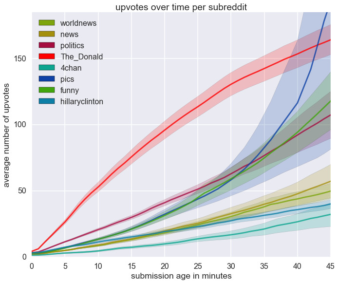
<p><img src="https://www.ryancompton.net/assets/reddit_scrape/ups_per_subreddit.jpg" alt="avg-votes" height="389px" width="480px" /></p>

<!--more-->

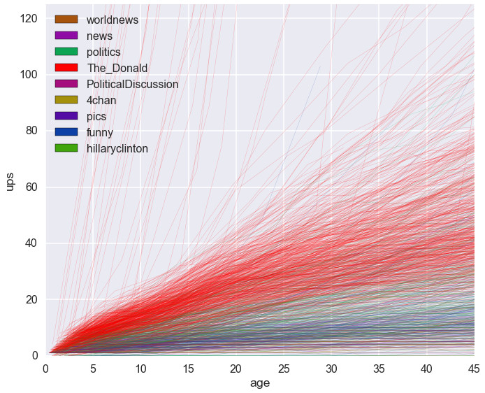
<p>The data was collected by polling <code class="language-plaintext highlighter-rouge">/new/</code> every 2 minutes for each subreddit over the past 3 days (2942138 records were found). The vast majority of submissions to reddit never get anywhere - I removed submissions which never attained over 50 upvotes which left me with 154160 records. The raw data is shown below:</p>

<p><img src="https://www.ryancompton.net/assets/reddit_scrape/ups_per_subreddit_raw.jpg" alt="raw-votes" height="389px" width="480px" /></p>

<p>Ranking on reddit is determined using a combination of upvotes, downvotes, and the age of the post at the time of each vote (cf. <a href="https://medium.com/hacking-and-gonzo/how-reddit-ranking-algorithms-work-ef111e33d0d9#.2t9s2cn3k">here</a>, <a href="http://scienceblogs.com/builtonfacts/2013/01/16/the-mathematics-of-reddit-rankings-or-how-upvotes-are-time-travel/">here</a>, and <a href="https://web.archive.org/web/20160407110929/http://www.redditblog.com/2009/10/reddits-new-comment-sorting-system.html">here</a> for some good explanations). In short, the ranking of a submission is set by the rating function</p>

\[\begin{equation*}
f(n,t) = 45000\log_{10}(n) + t
\end{equation*}\]

<p>where $n$ is the difference between upvotes and downvotes and $t$ is the number of seconds which elapsed between the post’s creation time and 7:46:43 am December 8th, 2005.</p>

<p>More recent posts have a larger $t$ which translates to a better ranking. Additionally, due to the shape of $\log_{10}$, votes matter substantially more when the number of upvotes nearly equals the number of downvotes (eg. when the post is brand new). Thus, the best way to get your post to the front page is to upvote aggressively when the post is very young.</p>

<p>My data suggests that members of <a href="https://www.reddit.com/r/The_Donald/comments/4oo3up/the_new_algorithm_is_a_totally_impartial_and_fair/">/r/The_Donald</a> are aware of this which explains why their new submissions have so many more upvotes despite the fact that competing subreddits in the plot are several orders of magnitude larger.</p>]]></content><author><name>Ryan Compton</name><email>ryan@ryancompton.net</email></author><category term="coding" /><summary type="html"><![CDATA[Here’s a plot of the cumulative number of upvotes per minute for submissions to a few major subreddits:]]></summary></entry><entry><title type="html">Taxi Strava</title><link href="https://www.ryancompton.net/2016/06/11/taxi-strava.html" rel="alternate" type="text/html" title="Taxi Strava" /><published>2016-06-11T00:00:00+00:00</published><updated>2016-06-11T00:00:00+00:00</updated><id>https://www.ryancompton.net/2016/06/11/taxi-strava</id><content type="html" xml:base="https://www.ryancompton.net/2016/06/11/taxi-strava.html"><![CDATA[<p>Last year <a href="http://chriswhong.com/">Chris Whong</a> used a <a href="http://www.dos.ny.gov/coog/foil2.html">foil</a> request to obtain a dataset with information on the locations, times, and medallions for 173 million NYC cab rides. I’m interested is determining which cabs are the fastest cabs are and how quickly they can get between various parts of the city.</p>

<!--more-->

<h2 id="data">Data</h2>

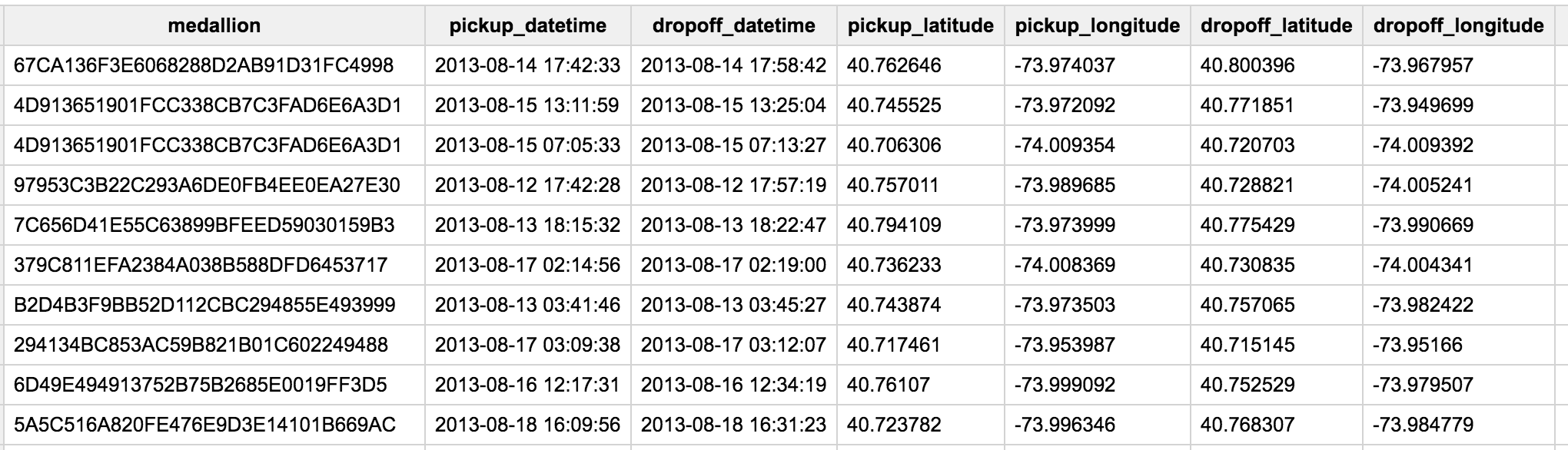
<p>Reddit users imjasonh and fhoffa parsed the raw data and loaded it into <a href="https://bigquery.cloud.google.com/table/imjasonh-storage:nyctaxi.trip_fare">a public BigQuery table</a> (<a href="https://bigquery.cloud.google.com/table/nyc-tlc:yellow.trips">another version</a> is also available from the NYC Taxi and Limousine Commission) The schema looks like:</p>

<p><img src="https://www.ryancompton.net/assets/taxi-strava/schema.png" alt="schema" /></p>

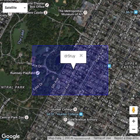
<p>As you can see, each ride has very specific details on pickup/dropoff locations as well as start/end times. I am interested in answering questions along the lines of “How fast do cabs get to the Flatiron from the Upper East Side?” which is hard to do from precise latitudes and longitudes. To rectify this I took a 6-character <a href="https://en.wikipedia.org/wiki/Geohash">geohash</a> of every pickup and dropoff location. A 6-character geohash buckets together coordinates that are within 0.61km of each other which allowed me to easily aggregate popular routes. An example is shown below (image from <a href="http://www.movable-type.co.uk/scripts/geohash.html">movable-type</a>):</p>

<p><img src="https://www.ryancompton.net/assets/taxi-strava/geohash-example.jpg" alt="geohash-example" /></p>

<p>The actual computations were done in Javascript using <a href="https://github.com/davetroy/geohash-js">https://github.com/davetroy/geohash-js</a> via a BigQuery UDF.</p>

<p>To make things more human readable, I used the <a href="http://www.geonames.org/maps/us-reverse-geocoder.html#findNearestIntersection">geonames api</a> to map the center of each bucket to an intersection. Not every geohash could be mapped to an intersection this way and those trips were dropped. Data was further cleaned by dropping trips using <code class="language-plaintext highlighter-rouge">(hack_license != "0") AND (hack_license != "CFCD208495D565EF66E7DFF9F98764DA")</code> which was observed in <a href="https://www.reddit.com/r/bigquery/comments/28ialf/173_million_2013_nyc_taxi_rides_shared_on_bigquery">a discussion</a> about the dataset.</p>

<p>This leaves us with a dataset of 158,320,608 cab rides bucketed into 32,654 distinct start/end points.</p>

<h2 id="results">Results</h2>

<p><em>Note: The 999th quantile for a trip’s average speed is 49.4289 mph - one trip had an average speed of 236,986,708 mph (roughly one third the speed of light). I removed any trip with average speed over 60mph from the data.</em></p>

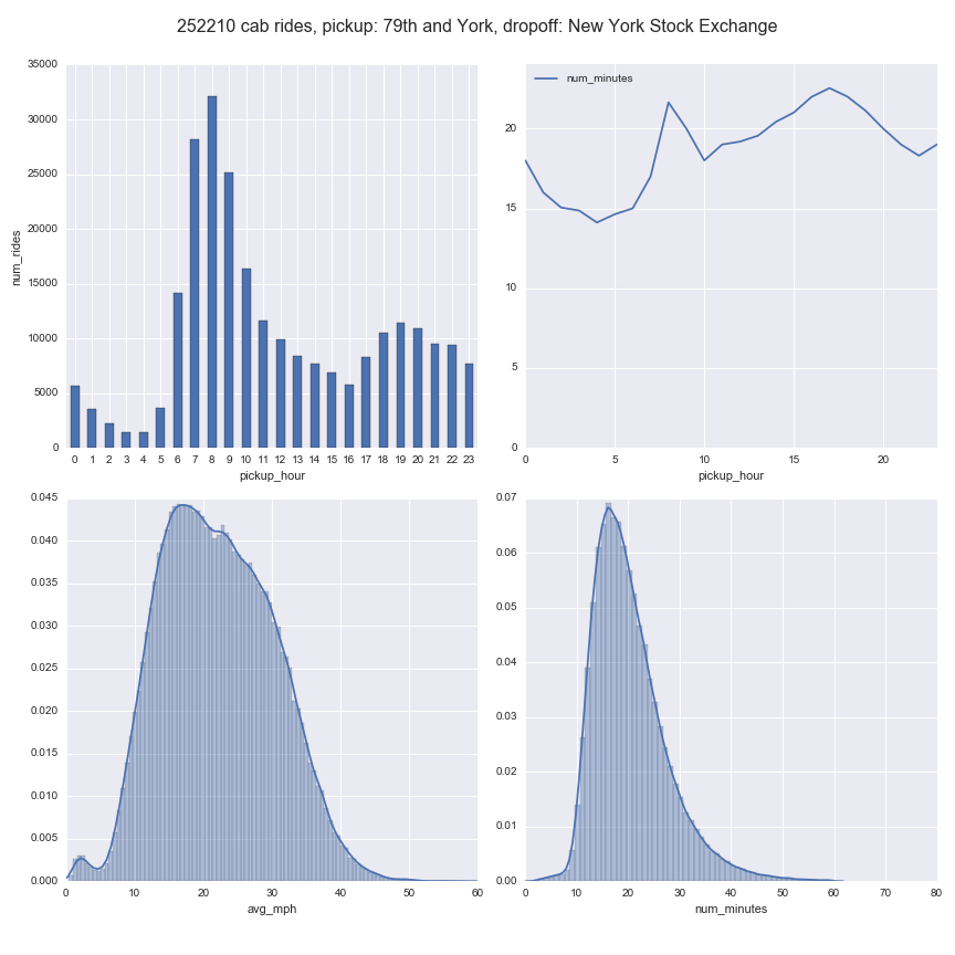
<p><strong>It takes ~20 minutes to get from 79th and York to the NYSE</strong></p>

<p>The taxi stand at East 79th Street and York Avenue has been taking residents of the Upper East Side to Wall Street since 1987. It has <a href="http://www.yelp.com/biz/79th-and-york-cab-share-new-york">4 stars on Yelp</a>. Each cab moves <a href="http://www.nyc.gov/html/tlc/downloads/pdf/group_ride_commission_presentation_x90_06-18-10.pdf">2 or more passengers at a fare of $6</a></p>

<p>I found 252,210 trips along this route in my data. On average cabs take 20.35 minutes and move at 22.11 mph. Of course you’ll go faster at 4am but most people don’t start their commute until 6 or 7am:</p>

<p><img src="https://www.ryancompton.net/assets/taxi-strava/taxi79th.png" alt="taxi79th" /></p>

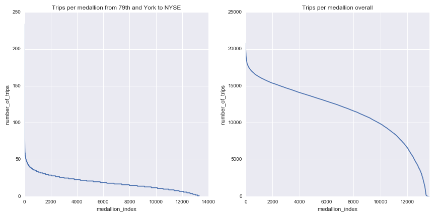
<p>Of the 13,347 medallions only a few regularly make the trip from 79th and York to Wall Street. The most dedicated cab drove the route 234 times over the year (only 7 drove it over 100 times):</p>

<p><img src="https://www.ryancompton.net/assets/taxi-strava/trips_per_medallion.png" alt="taxi79th" /></p>

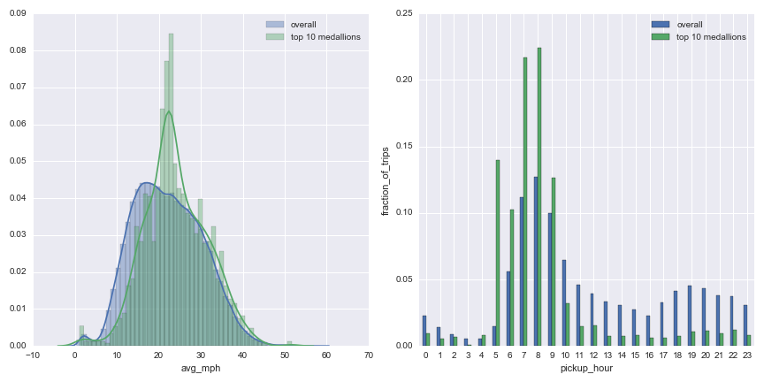
<p>The top 10 most frequent cab share drivers don’t go any faster than most though their average speed is more predictable (probably due to the fact that they often drive at the same time each day).
Additionally, when one uses the morning cab share they are far more likely to be picked up by a usual (especially at 5am):</p>

<p><img src="https://www.ryancompton.net/assets/taxi-strava/usuals_vs_overalls.png" alt="taxi79th" /></p>

<p>TODO:</p>

<figure class="highlight"><pre><code class="language-sql" data-lang="sql"><span class="k">SELECT</span>
  <span class="n">pickup_street1</span><span class="p">,</span> <span class="n">pickup_street2</span><span class="p">,</span> <span class="n">dropoff_street1</span><span class="p">,</span> <span class="n">dropoff_street2</span><span class="p">,</span>
  <span class="n">trips_medallion</span><span class="p">,</span> <span class="n">trips_pickup_datetime</span><span class="p">,</span> <span class="n">trips_dropoff_datetime</span><span class="p">,</span>
  <span class="n">ROUND</span><span class="p">(</span><span class="n">trips_avg_mph</span><span class="p">,</span><span class="mi">4</span><span class="p">)</span> <span class="k">AS</span> <span class="n">avg_mpg</span><span class="p">,</span>
  <span class="n">ROUND</span><span class="p">(</span><span class="n">trips_trip_duration_hours</span><span class="p">,</span><span class="mi">4</span><span class="p">)</span> <span class="k">AS</span> <span class="n">num_hours</span>
<span class="k">FROM</span>
  <span class="p">[</span><span class="n">taxi_strava</span><span class="p">.</span><span class="n">joined_geohash_geonames</span><span class="p">]</span>
<span class="k">WHERE</span>
  <span class="n">trips_geohashed_dropoff</span> <span class="o">=</span> <span class="s1">'dr5ru2'</span>
  <span class="k">AND</span> <span class="n">trips_geohashed_pickup</span> <span class="o">=</span> <span class="s1">'dr5rvj'</span></code></pre></figure>]]></content><author><name>Ryan Compton</name><email>ryan@ryancompton.net</email></author><category term="coding" /><summary type="html"><![CDATA[Last year Chris Whong used a foil request to obtain a dataset with information on the locations, times, and medallions for 173 million NYC cab rides. I’m interested is determining which cabs are the fastest cabs are and how quickly they can get between various parts of the city.]]></summary></entry><entry><title type="html">What convolutional neural networks look at when they look at nudity</title><link href="https://www.ryancompton.net/2016/04/19/what-convolutional-neural-networks-look-at-when-they-look-at-nudity.html" rel="alternate" type="text/html" title="What convolutional neural networks look at when they look at nudity" /><published>2016-04-19T00:00:00+00:00</published><updated>2016-04-19T00:00:00+00:00</updated><id>https://www.ryancompton.net/2016/04/19/what-convolutional-neural-networks-look-at-when-they-look-at-nudity</id><content type="html" xml:base="https://www.ryancompton.net/2016/04/19/what-convolutional-neural-networks-look-at-when-they-look-at-nudity.html"><![CDATA[<p><em>Originally published on the Clarifai blog at <a href="http://blog.clarifai.com/what-convolutional-neural-networks-see-at-when-they-see-nudity/">http://blog.clarifai.com/what-convolutional-neural-networks-see-at-when-they-see-nudity/</a></em></p>

<p>Last week at Clarifai we <a href="http://blog.clarifai.com/moderate-filter-or-curate-adult-content-with-clarifais-nsfw-model/">formally</a> <a href="http://blog.clarifai.com/how-to-use-clarifai-to-protect-your-eyes-from-seeing-something-they-cant-unsee/">announced</a> our Not Safe for Work (NSFW) adult content recognition model. Automating the discovery of nude pictures has been a central problem in computer vision for over two decades now and, because of it’s rich history and straightforward goal, serves as a great example of how the field has evolved. In this blog post, I’ll use the problem of nudity detection to illustrate how training modern convolutional neural networks (convnets) differs from research done in the past.</p>

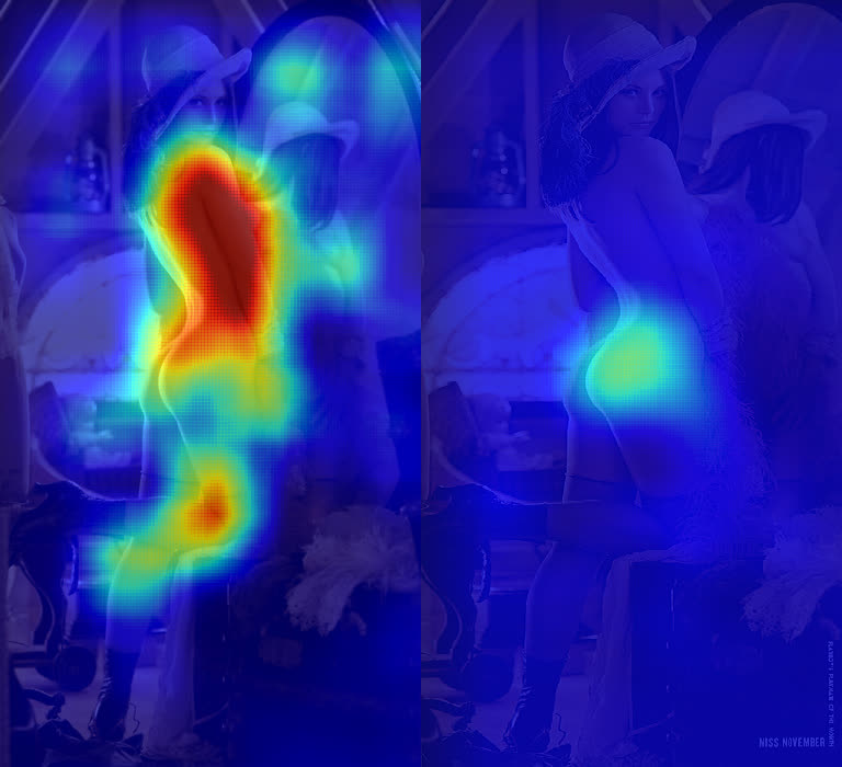
<p><img src="https://www.ryancompton.net/assets/pix/lena_heatmap.jpg" alt="Lenna heatmap" /></p>

<p>(<strong>Warning &amp; Disclaimer</strong>: This post contains visualizations of nudity for scientific purposes. Read no further if you are under the age of 18 or if you are offended by nudity.)</p>

<!--more-->

<h2 id="1996">1996</h2>

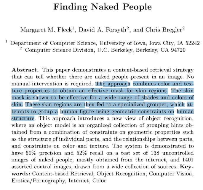
<p><img src="https://www.ryancompton.net/assets/pix/finding_naked_title.jpg" alt="Finding naked title" /></p>

<p>A seminal work in this field is the aptly-named “Finding Naked People” by Fleck et at.. It was published in the mid 90s and provides a good example of the kind of work that computer vision researchers would do prior to the convnet takeover. In section 2 of the paper the summarize the technique:</p>

<blockquote>
  <p>The algorithm:</p>
  <ul>
    <li>first locates images containing large areas of skin-colored region;</li>
    <li>then, within these areas, finds elongated regions and groups them into possible human limbs and connected groups of limbs, using specialized groupers which incorporate substantial amounts of information about object structure</li>
  </ul>
</blockquote>

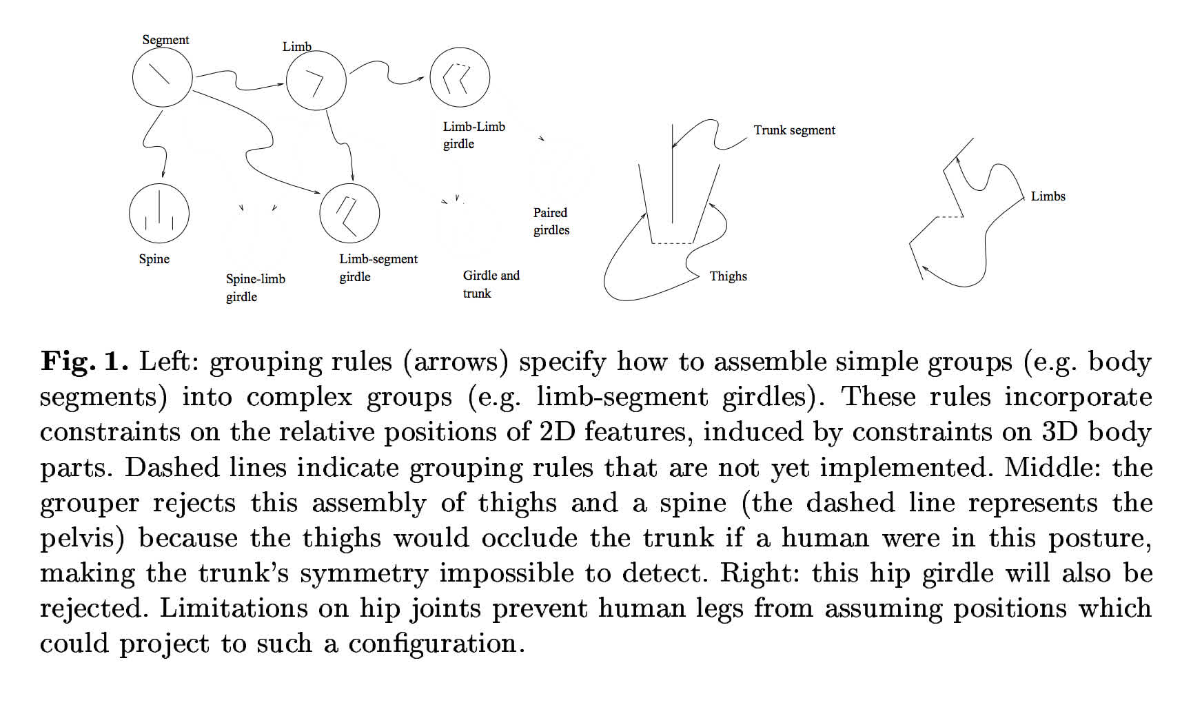
<p>Skin-detection is done by filtering in color space (note: HSV usually works well here but this paper implemented a specialized transformation of RGB) and grouping skin regions is done by modeling the the human figure “as an assembly  of nearly cylindrical parts, where both the individual geometry of the parts and the relationships between parts are constrained by the geometry of the skeleton” (cf. section 2). To get a better idea of the engineering that goes into building an algorithm like this we turn to fig. 1 in the paper where the authors illustrate a few of their handbuilt grouping rules:</p>

<p><img src="https://www.ryancompton.net/assets/pix/
finding_naked_figure.jpg" alt="Finding naked figure" /></p>

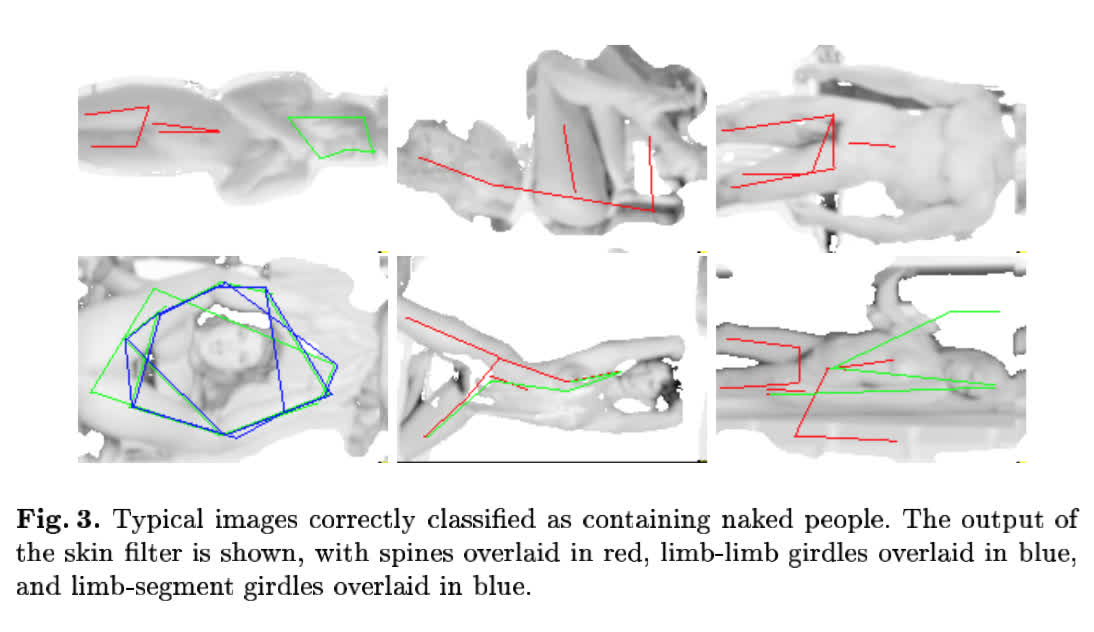
<p>The paper reports “60% precision and 52% recall on a test set of 138 uncontrolled images of naked people”. They also provide examples of true positives and false positives with visualizations of the features discovered by the algorithm overlaid:</p>

<p><img src="https://www.ryancompton.net/assets/pix/finding_naked_good.jpg" alt="Finding naked good" /></p>

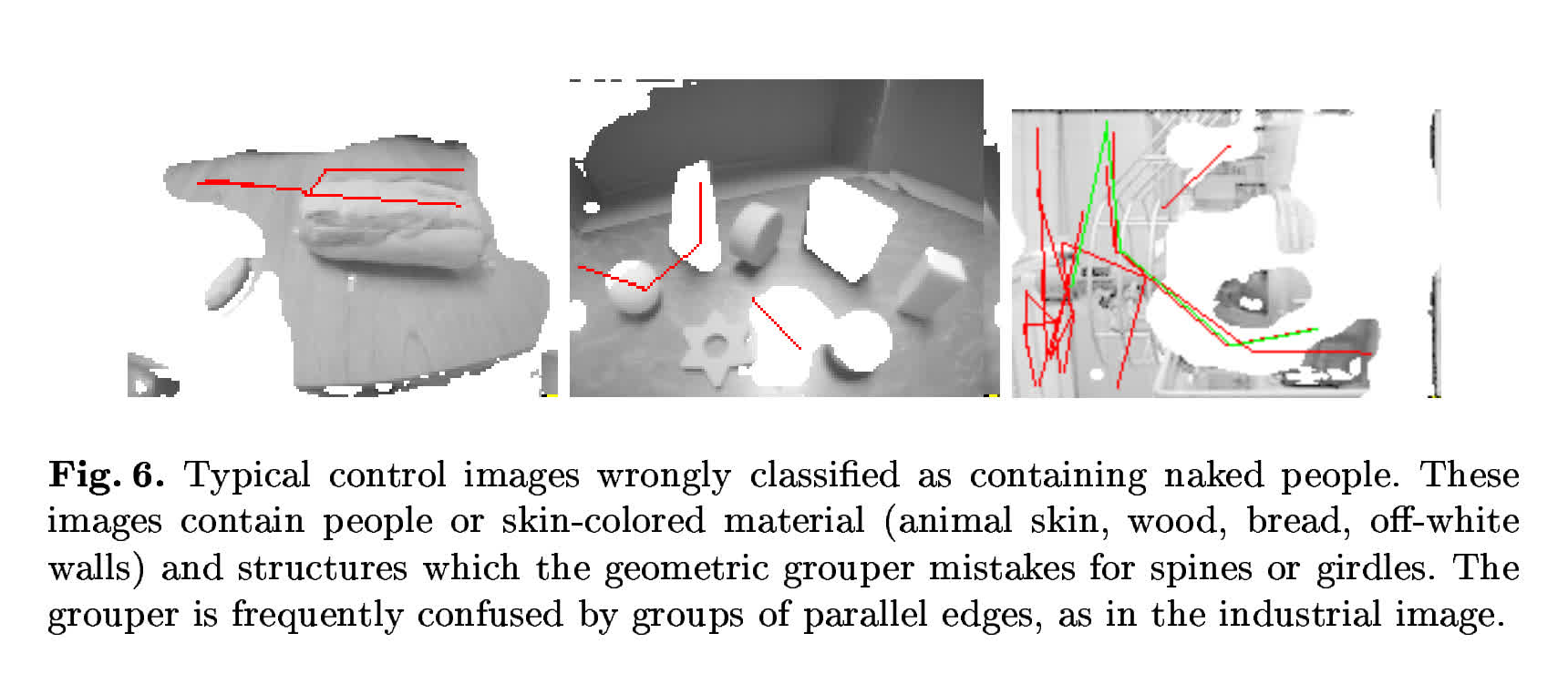
<p><img src="https://www.ryancompton.net/assets/pix/finding_naked_problems.jpg" alt="Finding naked problems" /></p>

<p>A major issue with building features by hand is that their complexity is limited by the patience and imagination of the researchers. In the next section, we’ll see how a convnet trained to perform the same task can learn much more sophisticated representations of the same data.</p>

<h2 id="2014">2014</h2>

<p>Instead of devising formal rules to describe how the input data should be represented, deep learning researchers devise network architectures and datasets which enable an A.I. system to learn representations directly from the data. However, since deep learning researchers don’t specify exactly how the network should behave on a given input, a new problem arises: How can one understand what the convolutional networks are activating on?</p>

<p><img src="https://www.ryancompton.net/assets/pix/zeiler_fergus.jpg" alt="ZF net" /></p>

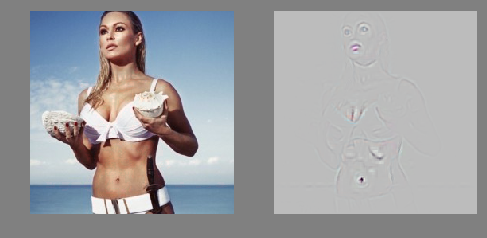
<p>Understanding the operation of a convnet requires interpreting the feature activity in various layers. In the rest of this post we’ll examine an early version of our NSFW model by mapping activities from the top layer back down to the input pixel space. This will allow us to see what input pattern originally caused a given activation in the feature maps (ie. why an image was flagged as “NSFW”).</p>

<h3 id="occulsion-sensitivity">Occulsion Sensitivity</h3>

<p>The image at the top of the post shows photos of <a href="https://en.wikipedia.org/wiki/Lenna">Lena Söderberg</a> after 64x64 sliding windows with a stride of 3 have applied of our nsfw model to cropped/occuluded versions of the raw image.</p>

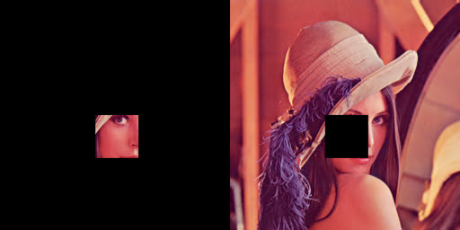
<p>To build the heatmap on the left we send each window to our convnet and average the “NSFW” scores over each pixel. When the convnet sees a crop filled with skin it tends to predict “NSFW” which leads to large red regions over Lena’s body. To create the heatmap on the right we systematically occlude parts of the raw image and report 1 minus the average “NSFW” scores (i.e. the “SFW” score). When the most NSFW regions are occluded the “SFW” scores increase and we see higher values in the heatmap. To be clear, the below figures have examples of what kind of images were fed into the convnet for each of two experiments above:</p>

<p><img src="https://www.ryancompton.net/assets/pix/lfaceblack.jpg" alt="Occulsions" /></p>

<p>One of the nice things about these occlusion experiments is that they’re possible to perform when the classifier is a complete black box. Here’s a code snippet that reproduces these results via our API:</p>

<figure class="highlight"><pre><code class="language-python" data-lang="python"><span class="c1"># NSFW occulsion experiment
</span>
<span class="kn">from</span> <span class="n">StringIO</span> <span class="kn">import</span> <span class="n">StringIO</span>

<span class="kn">import</span> <span class="n">matplotlib.pyplot</span> <span class="k">as</span> <span class="n">plt</span>
<span class="kn">import</span> <span class="n">numpy</span> <span class="k">as</span> <span class="n">np</span>
<span class="kn">from</span> <span class="n">PIL</span> <span class="kn">import</span> <span class="n">Image</span><span class="p">,</span> <span class="n">ImageDraw</span>
<span class="kn">import</span> <span class="n">requests</span>
<span class="kn">import</span> <span class="n">scipy.sparse</span> <span class="k">as</span> <span class="n">sp</span>

<span class="kn">from</span> <span class="n">clarifai.client</span> <span class="kn">import</span> <span class="n">ClarifaiApi</span>

<span class="n">CLARIFAI_APP_ID</span> <span class="o">=</span> <span class="sh">'</span><span class="s">...</span><span class="sh">'</span>
<span class="n">CLARIFAI_APP_SECRET</span> <span class="o">=</span> <span class="sh">'</span><span class="s">...</span><span class="sh">'</span>
<span class="n">clarifai</span> <span class="o">=</span> <span class="nc">ClarifaiApi</span><span class="p">(</span><span class="n">app_id</span><span class="o">=</span><span class="n">CLARIFAI_APP_ID</span><span class="p">,</span>
                       <span class="n">app_secret</span><span class="o">=</span><span class="n">CLARIFAI_APP_SECRET</span><span class="p">,</span>
                       <span class="n">base_url</span><span class="o">=</span><span class="sh">'</span><span class="s">https://api.clarifai.com</span><span class="sh">'</span><span class="p">)</span>

<span class="k">def</span> <span class="nf">batch_request</span><span class="p">(</span><span class="n">imgs</span><span class="p">,</span> <span class="n">bboxes</span><span class="p">):</span>
  <span class="sh">"""</span><span class="s">use the API to tag a batch of occulded images</span><span class="sh">"""</span>
  <span class="k">assert</span> <span class="nf">len</span><span class="p">(</span><span class="n">bboxes</span><span class="p">)</span> <span class="o">&lt;</span> <span class="mi">128</span>
  <span class="c1">#convert to image bytes
</span>  <span class="n">stringios</span> <span class="o">=</span> <span class="p">[]</span>
  <span class="k">for</span> <span class="n">img</span> <span class="ow">in</span> <span class="n">imgs</span><span class="p">:</span>
    <span class="n">stringio</span> <span class="o">=</span> <span class="nc">StringIO</span><span class="p">()</span>
    <span class="n">img</span><span class="p">.</span><span class="nf">save</span><span class="p">(</span><span class="n">stringio</span><span class="p">,</span> <span class="nb">format</span><span class="o">=</span><span class="sh">'</span><span class="s">JPEG</span><span class="sh">'</span><span class="p">)</span>
    <span class="n">stringios</span><span class="p">.</span><span class="nf">append</span><span class="p">(</span><span class="n">stringio</span><span class="p">)</span>
  <span class="c1">#call api and parse response
</span>  <span class="n">output</span> <span class="o">=</span> <span class="p">[]</span>
  <span class="n">response</span> <span class="o">=</span> <span class="n">clarifai</span><span class="p">.</span><span class="nf">tag_images</span><span class="p">(</span><span class="n">stringios</span><span class="p">,</span> <span class="n">model</span><span class="o">=</span><span class="sh">'</span><span class="s">nsfw-v1.0</span><span class="sh">'</span><span class="p">)</span>
  <span class="k">for</span> <span class="n">result</span><span class="p">,</span><span class="n">bbox</span> <span class="ow">in</span> <span class="nf">zip</span><span class="p">(</span><span class="n">response</span><span class="p">[</span><span class="sh">'</span><span class="s">results</span><span class="sh">'</span><span class="p">],</span> <span class="n">bboxes</span><span class="p">):</span>
    <span class="n">nsfw_idx</span> <span class="o">=</span> <span class="n">result</span><span class="p">[</span><span class="sh">'</span><span class="s">result</span><span class="sh">'</span><span class="p">][</span><span class="sh">'</span><span class="s">tag</span><span class="sh">'</span><span class="p">][</span><span class="sh">'</span><span class="s">classes</span><span class="sh">'</span><span class="p">].</span><span class="nf">index</span><span class="p">(</span><span class="sh">"</span><span class="s">sfw</span><span class="sh">"</span><span class="p">)</span>
    <span class="n">nsfw_score</span> <span class="o">=</span> <span class="n">result</span><span class="p">[</span><span class="sh">'</span><span class="s">result</span><span class="sh">'</span><span class="p">][</span><span class="sh">'</span><span class="s">tag</span><span class="sh">'</span><span class="p">][</span><span class="sh">'</span><span class="s">probs</span><span class="sh">'</span><span class="p">][</span><span class="n">nsfw_idx</span><span class="p">]</span>
    <span class="n">output</span><span class="p">.</span><span class="nf">append</span><span class="p">((</span><span class="n">nsfw_score</span><span class="p">,</span> <span class="n">bbox</span><span class="p">))</span>
  <span class="k">return</span> <span class="n">output</span>

<span class="k">def</span> <span class="nf">build_bboxes</span><span class="p">(</span><span class="n">img</span><span class="p">,</span> <span class="n">boxsize</span><span class="o">=</span><span class="mi">72</span><span class="p">,</span> <span class="n">stride</span><span class="o">=</span><span class="mi">25</span><span class="p">):</span>
  <span class="sh">"""</span><span class="s">Generate all the bboxes used in the experiment</span><span class="sh">"""</span>
  <span class="n">width</span> <span class="o">=</span> <span class="n">boxsize</span>
  <span class="n">height</span> <span class="o">=</span> <span class="n">boxsize</span>
  <span class="n">bboxes</span> <span class="o">=</span> <span class="p">[]</span>
  <span class="k">for</span> <span class="n">top</span> <span class="ow">in</span> <span class="nf">range</span><span class="p">(</span><span class="mi">0</span><span class="p">,</span> <span class="n">img</span><span class="p">.</span><span class="n">size</span><span class="p">[</span><span class="mi">1</span><span class="p">],</span> <span class="n">stride</span><span class="p">):</span>
    <span class="k">for</span> <span class="n">left</span> <span class="ow">in</span> <span class="nf">range</span><span class="p">(</span><span class="mi">0</span><span class="p">,</span> <span class="n">img</span><span class="p">.</span><span class="n">size</span><span class="p">[</span><span class="mi">0</span><span class="p">],</span> <span class="n">stride</span><span class="p">):</span>
      <span class="n">bboxes</span><span class="p">.</span><span class="nf">append</span><span class="p">((</span><span class="n">left</span><span class="p">,</span> <span class="n">top</span><span class="p">,</span> <span class="n">left</span><span class="o">+</span><span class="n">width</span><span class="p">,</span> <span class="n">top</span><span class="o">+</span><span class="n">height</span><span class="p">))</span>
  <span class="k">return</span> <span class="n">bboxes</span>

<span class="k">def</span> <span class="nf">draw_occulsions</span><span class="p">(</span><span class="n">img</span><span class="p">,</span> <span class="n">bboxes</span><span class="p">):</span>
  <span class="sh">"""</span><span class="s">Overlay bboxes on the test image</span><span class="sh">"""</span>
  <span class="n">images</span> <span class="o">=</span> <span class="p">[]</span>
  <span class="k">for</span> <span class="n">bbox</span> <span class="ow">in</span> <span class="n">bboxes</span><span class="p">:</span>
    <span class="n">img2</span> <span class="o">=</span> <span class="n">img</span><span class="p">.</span><span class="nf">copy</span><span class="p">()</span>
    <span class="n">draw</span> <span class="o">=</span> <span class="n">ImageDraw</span><span class="p">.</span><span class="nc">Draw</span><span class="p">(</span><span class="n">img2</span><span class="p">)</span>
    <span class="n">draw</span><span class="p">.</span><span class="nf">rectangle</span><span class="p">(</span><span class="n">bbox</span><span class="p">,</span> <span class="n">fill</span><span class="o">=</span><span class="bp">True</span><span class="p">)</span>
    <span class="n">images</span><span class="p">.</span><span class="nf">append</span><span class="p">(</span><span class="n">img2</span><span class="p">)</span>
  <span class="k">return</span> <span class="n">images</span>

<span class="k">def</span> <span class="nf">alpha_composite</span><span class="p">(</span><span class="n">img</span><span class="p">,</span> <span class="n">heatmap</span><span class="p">):</span>
  <span class="sh">"""</span><span class="s">Blend a PIL image and a numpy array corresponding to a heatmap in a nice way</span><span class="sh">"""</span>
  <span class="k">if</span> <span class="n">img</span><span class="p">.</span><span class="n">mode</span> <span class="o">==</span> <span class="sh">'</span><span class="s">RBG</span><span class="sh">'</span><span class="p">:</span>
    <span class="n">img</span><span class="p">.</span><span class="nf">putalpha</span><span class="p">(</span><span class="mi">100</span><span class="p">)</span>
  <span class="n">cmap</span> <span class="o">=</span> <span class="n">plt</span><span class="p">.</span><span class="nf">get_cmap</span><span class="p">(</span><span class="sh">'</span><span class="s">jet</span><span class="sh">'</span><span class="p">)</span>
  <span class="n">rgba_img</span> <span class="o">=</span> <span class="nf">cmap</span><span class="p">(</span><span class="n">heatmap</span><span class="p">)</span>
  <span class="n">rgba_img</span><span class="p">[:,:,:][:]</span> <span class="o">=</span> <span class="mf">0.7</span> <span class="c1">#alpha overlay
</span>  <span class="n">rgba_img</span> <span class="o">=</span> <span class="n">Image</span><span class="p">.</span><span class="nf">fromarray</span><span class="p">(</span><span class="n">np</span><span class="p">.</span><span class="nf">uint8</span><span class="p">(</span><span class="nf">cmap</span><span class="p">(</span><span class="n">heatmap</span><span class="p">)</span><span class="o">*</span><span class="mi">255</span><span class="p">))</span>
  <span class="k">return</span> <span class="n">Image</span><span class="p">.</span><span class="nf">blend</span><span class="p">(</span><span class="n">img</span><span class="p">,</span> <span class="n">rgba_img</span><span class="p">,</span> <span class="mf">0.8</span><span class="p">)</span>

<span class="k">def</span> <span class="nf">get_nsfw_occlude_mask</span><span class="p">(</span><span class="n">img</span><span class="p">,</span> <span class="n">boxsize</span><span class="o">=</span><span class="mi">64</span><span class="p">,</span> <span class="n">stride</span><span class="o">=</span><span class="mi">25</span><span class="p">):</span>
  <span class="sh">"""</span><span class="s">generate bboxes and occluded images, call the API, blend the results together</span><span class="sh">"""</span>
  <span class="n">bboxes</span> <span class="o">=</span> <span class="nf">build_bboxes</span><span class="p">(</span><span class="n">img</span><span class="p">,</span> <span class="n">boxsize</span><span class="o">=</span><span class="n">boxsize</span><span class="p">,</span> <span class="n">stride</span><span class="o">=</span><span class="n">stride</span><span class="p">)</span>
  <span class="k">print</span> <span class="sh">'</span><span class="s">api calls needed:{}</span><span class="sh">'</span><span class="p">.</span><span class="nf">format</span><span class="p">(</span><span class="nf">len</span><span class="p">(</span><span class="n">bboxes</span><span class="p">))</span>
  <span class="n">scored_bboxes</span> <span class="o">=</span> <span class="p">[]</span>
  <span class="n">batch_size</span> <span class="o">=</span> <span class="mi">125</span>
  <span class="k">for</span> <span class="n">i</span> <span class="ow">in</span> <span class="nf">range</span><span class="p">(</span><span class="mi">0</span><span class="p">,</span> <span class="nf">len</span><span class="p">(</span><span class="n">bboxes</span><span class="p">),</span> <span class="n">batch_size</span><span class="p">):</span>
    <span class="n">bbox_batch</span> <span class="o">=</span> <span class="n">bboxes</span><span class="p">[</span><span class="n">i</span><span class="p">:</span><span class="n">i</span> <span class="o">+</span> <span class="n">batch_size</span><span class="p">]</span>
    <span class="n">occluded_images</span> <span class="o">=</span> <span class="nf">draw_occulsions</span><span class="p">(</span><span class="n">img</span><span class="p">,</span> <span class="n">bbox_batch</span><span class="p">)</span>
    <span class="n">results</span> <span class="o">=</span> <span class="nf">batch_request</span><span class="p">(</span><span class="n">occluded_images</span><span class="p">,</span> <span class="n">bbox_batch</span><span class="p">)</span>
    <span class="n">scored_bboxes</span><span class="p">.</span><span class="nf">extend</span><span class="p">(</span><span class="n">results</span><span class="p">)</span>
  <span class="n">heatmap</span> <span class="o">=</span> <span class="n">np</span><span class="p">.</span><span class="nf">zeros</span><span class="p">(</span><span class="n">img</span><span class="p">.</span><span class="n">size</span><span class="p">)</span>
  <span class="n">sparse_masks</span> <span class="o">=</span> <span class="p">[]</span>
  <span class="k">for</span> <span class="n">idx</span><span class="p">,</span> <span class="p">(</span><span class="n">nsfw_score</span><span class="p">,</span> <span class="n">bbox</span><span class="p">)</span> <span class="ow">in</span> <span class="nf">enumerate</span><span class="p">(</span><span class="n">scored_bboxes</span><span class="p">):</span>
    <span class="n">mask</span> <span class="o">=</span> <span class="n">np</span><span class="p">.</span><span class="nf">zeros</span><span class="p">(</span><span class="n">img</span><span class="p">.</span><span class="n">size</span><span class="p">)</span>
    <span class="n">mask</span><span class="p">[</span><span class="n">bbox</span><span class="p">[</span><span class="mi">0</span><span class="p">]:</span><span class="n">bbox</span><span class="p">[</span><span class="mi">2</span><span class="p">],</span> <span class="n">bbox</span><span class="p">[</span><span class="mi">1</span><span class="p">]:</span><span class="n">bbox</span><span class="p">[</span><span class="mi">3</span><span class="p">]]</span> <span class="o">=</span> <span class="n">nsfw_score</span>
    <span class="n">Asp</span> <span class="o">=</span> <span class="n">sp</span><span class="p">.</span><span class="nf">csr_matrix</span><span class="p">(</span><span class="n">mask</span><span class="p">)</span>
    <span class="n">sparse_masks</span><span class="p">.</span><span class="nf">append</span><span class="p">(</span><span class="n">Asp</span><span class="p">)</span>
    <span class="n">heatmap</span> <span class="o">=</span> <span class="n">heatmap</span> <span class="o">+</span> <span class="p">(</span><span class="n">mask</span> <span class="o">-</span> <span class="n">heatmap</span><span class="p">)</span><span class="o">/</span><span class="p">(</span><span class="n">idx</span><span class="o">+</span><span class="mi">1</span><span class="p">)</span>    
  <span class="k">return</span> <span class="nf">alpha_composite</span><span class="p">(</span><span class="n">img</span><span class="p">,</span> <span class="mi">80</span><span class="o">*</span><span class="n">np</span><span class="p">.</span><span class="nf">transpose</span><span class="p">(</span><span class="n">heatmap</span><span class="p">)),</span> <span class="n">np</span><span class="p">.</span><span class="nf">stack</span><span class="p">(</span><span class="n">sparse_masks</span><span class="p">)</span>

<span class="c1">#Download full Lena image
</span><span class="n">r</span> <span class="o">=</span> <span class="n">requests</span><span class="p">.</span><span class="nf">get</span><span class="p">(</span><span class="sh">'</span><span class="s">https://clarifai-img.s3.amazonaws.com/blog/len_full.jpeg</span><span class="sh">'</span><span class="p">)</span>
<span class="n">stringio</span> <span class="o">=</span> <span class="nc">StringIO</span><span class="p">(</span><span class="n">r</span><span class="p">.</span><span class="n">content</span><span class="p">)</span>
<span class="n">img</span> <span class="o">=</span> <span class="n">Image</span><span class="p">.</span><span class="nf">open</span><span class="p">(</span><span class="n">stringio</span><span class="p">,</span> <span class="sh">'</span><span class="s">r</span><span class="sh">'</span><span class="p">)</span>
<span class="n">img</span><span class="p">.</span><span class="nf">putalpha</span><span class="p">(</span><span class="mi">1000</span><span class="p">)</span>

<span class="c1">#set boxsize and stride (warning! a low stride will lead to thousands of API calls)
</span><span class="n">boxsize</span><span class="o">=</span> <span class="mi">64</span>
<span class="n">stride</span><span class="o">=</span> <span class="mi">48</span>
<span class="n">blended</span><span class="p">,</span> <span class="n">masks</span> <span class="o">=</span> <span class="nf">get_nsfw_occlude_mask</span><span class="p">(</span><span class="n">img</span><span class="p">,</span> <span class="n">boxsize</span><span class="o">=</span><span class="n">boxsize</span><span class="p">,</span> <span class="n">stride</span><span class="o">=</span><span class="n">stride</span><span class="p">)</span>

<span class="c1">#viz
</span><span class="n">blended</span><span class="p">.</span><span class="nf">show</span><span class="p">()</span></code></pre></figure>

<p>While these kinds of experiments provide a straightforward way of displaying classifier outputs they have a drawback in that the visualizations produced are often quite blurry. This prevents us from gaining meaningful insight into what the network is actually doing and understanding what could have gone wrong during training.</p>

<h3 id="deconvolutional-networks">Deconvolutional Networks</h3>

<p>Once we’ve trained a network on a given dataset we’d like to be able to take an image and a class and ask the convnet something along the lines of “How can we change this image in order to look more like the given class?”. For this we use a deconvolutional network (deconvnet), cf section 2 from Zeiler and Fergus 2014:</p>

<blockquote>
  <p>A deconvnet can be thought of as a convnet model that uses the same components (filtering, pooling) but in reverse, so instead of mapping pixels to features does the opposite. To examine a given convnet activation, we set all other activations in
the layer to zero and pass the feature maps as input to the attached deconvnet layer. Then we successively (i) unpool, (ii) rectify and (iii) filter to reconstruct the activity in the layer beneath that gave rise to the chosen activation. This is
then repeated until input pixel space is reached.</p>
</blockquote>

<blockquote>
  <p>The procedure is similar to backpropping a single strong activation (rather than the usual gradients), i.e. computing $\frac{\partial h}{ \partial X_n}$ where $h$ is the element of the feature map with the strong activation and $X_n$ is the input image.</p>
</blockquote>

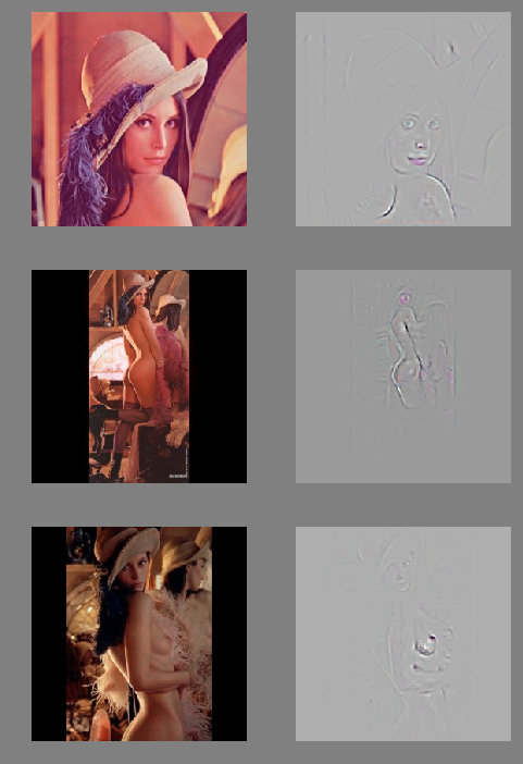
<p>Here is the result we get when using a deconvnet to visualize how we should modify photos of Lena to look more like pornography (note: the deconvnet used here needed a square image to function correctly - we padded the full Lena image to get the right aspect ratio):</p>

<p><img src="https://www.ryancompton.net/assets/pix/len_4x4.jpeg" alt="Lena 2x2" /></p>

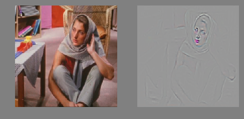
<p><a href="https://dsp.stackexchange.com/questions/18631/who-is-barbara-test-image">Barbara</a> is the G-rated version of Lena. According to our deconvnet, we could modify Barbara to look more PG by adding redness to her lips:</p>

<p><img src="https://www.ryancompton.net/assets/pix/barbara_deconv.jpeg" alt="Barbara" /></p>

<p>This image of <a href="https://en.wikipedia.org/wiki/Ursula_Andress">Ursula Andress</a> as Honey Rider in the James Bond film <em>Dr. No</em> was voted number one in “the 100 Greatest Sexy Moments in screen history” by a <a href="http://news.bbc.co.uk/2/hi/entertainment/3250386.stm">UK survey in 2003</a>:</p>

<p><img src="https://www.ryancompton.net/assets/pix/ursula_deconv.jpeg" alt="Ursula" /></p>

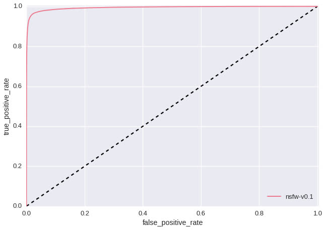
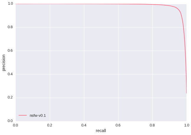
<p>A salient feature of the above experiments is that the convnet learned red lips and navels as indicative of “NSFW”. This likely means that we didn’t include enough images of red lips and navels in our “SFW” training data. Had we only evaluated our model by examining precision/recall and ROC curves (shown below - test set size: 428,271) we would have never discovered this issue as our test data would have the same shortcoming. This highlights a fundamental difference between training rule-based classifiers and modern A.I. research. Rather than redesigning features by hand, we redesign our training data until the discovered features are improved.</p>

<p><img src="https://www.ryancompton.net/assets/pix/roc.jpg" alt="ROC" /></p>

<p><img src="https://www.ryancompton.net/assets/pix/prec_recall.jpg" alt="PR" /></p>

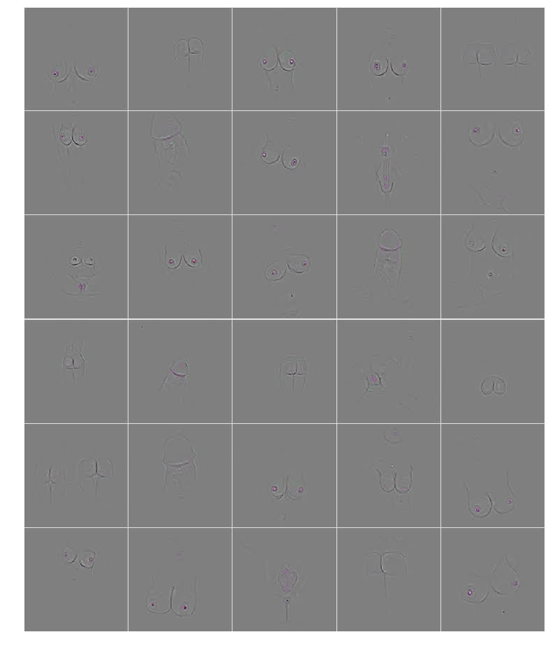
<p>Finally, as a sanity check, we run the deconvnet on hardcore porno to ensure that the learned feature activations do indeed to correspond to obviously nsfw objects:</p>

<p><img src="https://www.ryancompton.net/assets/pix/deconv_porno.jpg" alt="nsfw_grid" /></p>

<p>Here, we can clearly see that the convnet correctly learned penis, anus, vulva, nipple, and buttocks - objects which our model should flag. What’s more, the discovered features are far more detailed and complex than what researchers could design by hand which helps explain the major improvements we get by using convnets to recognize NSFW images.</p>

<p>If you’re interested in using convnets to filter NSFW images, check our NSFW API documentation to get started. <a href="https://developer.clarifai.com/guide/tag#nsfw">https://developer.clarifai.com/guide/tag#nsfw</a></p>]]></content><author><name>Ryan Compton</name><email>ryan@ryancompton.net</email></author><category term="coding" /><category term="machine learning" /><summary type="html"><![CDATA[Originally published on the Clarifai blog at http://blog.clarifai.com/what-convolutional-neural-networks-see-at-when-they-see-nudity/ Last week at Clarifai we formally announced our Not Safe for Work (NSFW) adult content recognition model. Automating the discovery of nude pictures has been a central problem in computer vision for over two decades now and, because of it’s rich history and straightforward goal, serves as a great example of how the field has evolved. In this blog post, I’ll use the problem of nudity detection to illustrate how training modern convolutional neural networks (convnets) differs from research done in the past. (Warning &amp; Disclaimer: This post contains visualizations of nudity for scientific purposes. Read no further if you are under the age of 18 or if you are offended by nudity.)]]></summary></entry><entry><title type="html">Darknet Market Basket Analysis</title><link href="https://www.ryancompton.net/2015/03/24/darknet-market-basket-analysis.html" rel="alternate" type="text/html" title="Darknet Market Basket Analysis" /><published>2015-03-24T00:00:00+00:00</published><updated>2015-03-24T00:00:00+00:00</updated><id>https://www.ryancompton.net/2015/03/24/darknet-market-basket-analysis</id><content type="html" xml:base="https://www.ryancompton.net/2015/03/24/darknet-market-basket-analysis.html"><![CDATA[<p>The <a href="https://en.wikipedia.org/wiki/Evolution_%28marketplace%29">Evolution darknet marketplace</a> was an online black market which operated from January 2014 until Wednesday of last week when it <a href="http://www.forbes.com/sites/thomasbrewster/2015/03/18/evolution-market-a-scam-says-site-pr/">suddenly disappeared</a>. A few days later, <a href="https://www.reddit.com/r/DarkNetMarkets/comments/2zllmv/evolution_market_mirrorscrapes_torrent_released/">in a reddit post</a>, <a href="http://www.gwern.net/">gwern</a> released a torrent containing daily wget crawls of the site dating back to its inception. I ran some off-the-shelf affinity analysis on the dataset – here’s what I found:</p>

<h3 id="products-can-be-categorized-based-on-who-sells-them"><em style="color: white">Products can be categorized based on who sells them</em></h3>

<p>On Evolution there are a few top-level categories (“Drugs”, “Digital Goods”, “Fraud Related” etc.) which are subdivided into product-specific pages. Each page contains several listings by various vendors.</p>

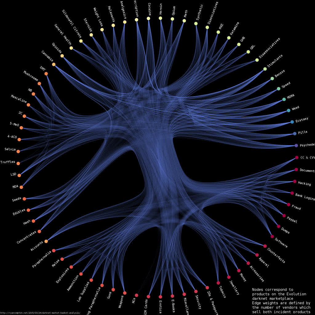
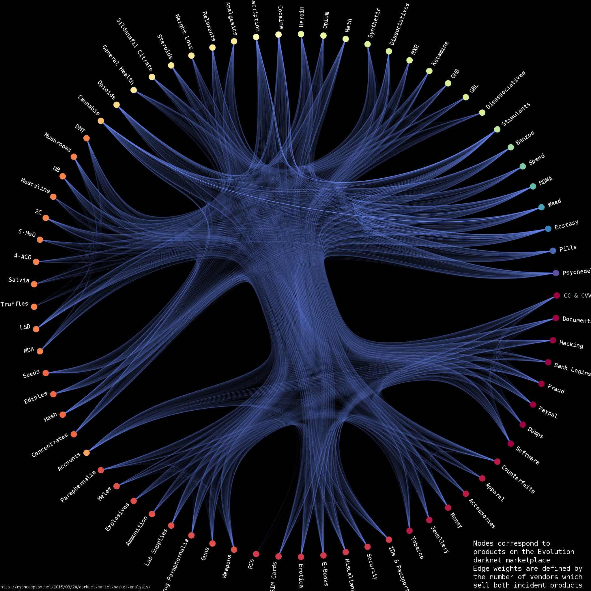
<p>I built a graph between products based on vendor co-occurrence relationships, i.e. each node corresponds to a product with edge weights defined by the number of vendors who sell both incident products. So, for example, if there are 3 vendors selling both mescaline and 4-AcO-DMT then my graph has an edge with weight 3 between the mescaline and 4-AcO-DMT nodes. I used <a href="https://graph-tool.skewed.de/static/doc/community.html#graph_tool.community.minimize_blockmodel_dl">graph-tool’s</a> implementation of stochastic block model-based hierarchal edge bundling to generate the below visualization of the Evolution product network:</p>

<p><img src="https://www.ryancompton.net/assets/darknet-market-basket-analysis/evo_market_labeled_new_1024.jpg" alt="evo_market_labeled_1024" /></p>

<p>The graph is available in graphml format <a href="https://www.ryancompton.net/assets/darknet-market-basket-analysis/evo_product_affinity.xml">here.</a> It contains 73 nodes and 2,219 edges (I found a total of 3,785 vendors in the data).</p>

<p>Edges with higher weights are drawn more brightly. Nodes are clustered with a <a href="http://arxiv.org/abs/1310.4377">stochastic block model</a> and nodes within the same cluster are assigned the same color. There is a clear division between the clusters on the top half of the graph (correpsonding to drugs) and the clusters on the bottom half (corresponding to non-drugs, i.e. weapons/hacking/credit cards/etc.). This suggests that vendors who sold drugs were not as likely to sell non-drugs and vice versa.</p>

<!--more-->

<p>I used a short python script to parse the scraped html and remove duplicate data, its available <a href="https://www.ryancompton.net/assets/darknet-market-basket-analysis/parse_evo.py">here</a>. It takes a while to go through the entire dataset (which is about 90GB); if you’d like to skip that you can download the results of my parse as a <a href="https://www.ryancompton.net/assets/darknet-market-basket-analysis/products_vendors.zip">.tsv file</a>. The plotting code is available as an <a href="https://www.ryancompton.net/assets/darknet-market-basket-analysis/draw_evo.html">ipython notebook</a>. High-res version of the above plot <a href="https://www.ryancompton.net/assets/darknet-market-basket-analysis/evo_market_labeled_new.jpg">here</a>.</p>

<h3 id="917-of-vendors-who-sold-speed-and-mdma-also-sold-ecstasy"><em style="color: white">91.7% of vendors who sold speed and MDMA also sold ecstasy</em></h3>

<p><a href="https://en.wikipedia.org/wiki/Association_rule_learning">Association rule learning</a> is a straightforward and popular way to solve problems in <a href="https://en.wikipedia.org/wiki/Affinity_analysis">market basket analysis</a>. The traditional application is to suggest items to shoppers based on what other customers are putting in their carts. For some reason the canonical example is “customers who buy diapers also buy beer”.</p>

<p>We don’t have customer data from a crawl of the public postings on Evolution. However, we do have data on what each vendor sells which can help us quantify results suggested by the visual analysis done above.</p>

<p>Here’s an example of what our database looks like (the complete file has 3,785 rows (one for each vendor)):</p>

<table>
  <thead>
    <tr>
      <th>Vendor</th>
      <th>Products</th>
    </tr>
  </thead>
  <tbody>
    <tr>
      <td>MrHolland</td>
      <td>[‘Cocaine’, ‘Cannabis’, ‘Stimulants’, ‘Hash’]</td>
    </tr>
    <tr>
      <td>Packstation24</td>
      <td>[‘Accounts’, ‘Benzos’, ‘IDs &amp; Passports’, ‘SIM Cards’, ‘Fraud’]</td>
    </tr>
    <tr>
      <td>Spinifex</td>
      <td>[‘Benzos’, ‘Cannabis’, ‘Cocaine’, ‘Stimulants’, ‘Prescription’, ‘Sildenafil Citrate’]</td>
    </tr>
    <tr>
      <td>OzVendor</td>
      <td>[‘Software’, ‘Erotica’, ‘Dumps’, ‘E-Books’, ‘Fraud’]</td>
    </tr>
    <tr>
      <td>OzzyDealsDirect</td>
      <td>[‘Cannabis’, ‘Seeds’, ‘MDMA’, ‘Weed’]</td>
    </tr>
    <tr>
      <td>TatyThai</td>
      <td>[‘Accounts’, ‘Documents &amp; Data’, ‘IDs &amp; Passports’, ‘Paypal’, ‘CC &amp; CVV’]</td>
    </tr>
    <tr>
      <td>PEA_King</td>
      <td>[‘Mescaline’, ‘Stimulants’, ‘Meth’, ‘Psychedelics’]</td>
    </tr>
    <tr>
      <td>PROAMFETAMINE</td>
      <td>[‘MDMA’, ‘Speed’, ‘Stimulants’, ‘Ecstasy’, ‘Pills’]</td>
    </tr>
    <tr>
      <td>ParrotFish</td>
      <td>[‘Weight Loss’, ‘Stimulants’, ‘Prescription’, ‘Ecstasy’]</td>
    </tr>
  </tbody>
</table>

<p>Before saying anything more about association rule learning here’s a quick glossary of terms:</p>

<ul>
  <li>The <strong>support</strong>, $supp(X)$, of an itemset, $X$, is defined as the proportion of transactions in the data set which contain $X$. In the table above, the support of ‘Cocaine’ is 2 because it appears in two vendors’ storefronts (MrHolland and Spinifex)</li>
  <li>The <strong>confidence</strong> of a rule is defined $\mathrm{conf}(X \Rightarrow Y) = \mathrm{supp}(X \cup Y) / \mathrm{supp}(X)$. In our example the confidence of the rule ‘Cannabis’ ==&gt; ‘Cocaine’ is 2/3 because out the 3 vendors who sell ‘Cannabis’ 2 of them sell ‘Cocaine’. The support of this rule is 2.</li>
</ul>

<p>Association rule mining is a huge field within computer science – hundreds (thousands?) of papers have been published over the past two decades. The necessary algorithms are very complex but open source implementations are available. My favorite collection (and the one I used for these experiments) is Philippe Fournier Viger’s <a href="http://www.philippe-fournier-viger.com/spmf/">spmf</a>.</p>

<p>I ran the FP-Growth algorithm with a minimum allowable support of 40 and a minimum allowable confidence of 0.1. The algorithm learned 12,364 rules. These can be downloaded as a .tsv <a href="https://www.ryancompton.net/assets/darknet-market-basket-analysis/learned_rules.tsv">here</a>. I’ve selected a few rules for display below:</p>

<table>
  <thead>
    <tr>
      <th>antecedent</th>
      <th>consequent</th>
      <th>support</th>
      <th>confidence</th>
    </tr>
  </thead>
  <tbody>
    <tr>
      <td>[‘Speed’, ‘MDMA’]</td>
      <td>[‘Ecstasy’]</td>
      <td>155</td>
      <td>0.91716</td>
    </tr>
    <tr>
      <td>[‘Ecstasy’, ‘Stimulants’]</td>
      <td>[‘MDMA’]</td>
      <td>310</td>
      <td>0.768</td>
    </tr>
    <tr>
      <td>[‘Speed’, ‘Weed’, ‘Stimulants’]</td>
      <td>[‘Cannabis’, ‘Ecstasy’]</td>
      <td>68</td>
      <td>0.623</td>
    </tr>
    <tr>
      <td>[‘Fraud’, ‘Hacking’]</td>
      <td>[‘Accounts’]</td>
      <td>53</td>
      <td>0.623</td>
    </tr>
    <tr>
      <td>[‘Fraud’, ‘CC &amp; CVV’, ‘Accounts’]</td>
      <td>[‘Paypal’]</td>
      <td>43</td>
      <td>0.492</td>
    </tr>
    <tr>
      <td>[‘Documents &amp; Data’]</td>
      <td>[‘Accounts’]</td>
      <td>139</td>
      <td>0.492</td>
    </tr>
    <tr>
      <td>[‘Guns’]</td>
      <td>[‘Weapons’]</td>
      <td>72</td>
      <td>0.98</td>
    </tr>
    <tr>
      <td>[‘Weapons’]</td>
      <td>[‘Guns’]</td>
      <td>72</td>
      <td>0.40</td>
    </tr>
  </tbody>
</table>

<h3 id="other-remarks"><em>Other Remarks</em></h3>

<p>I think I’ve only scratched the surface of what’s possible with this data. There are much more detailed product descriptions for each listing in the .tsv. That text is harder to work with so it will take some time to figure out what makes sense.</p>]]></content><author><name>Ryan Compton</name><email>ryan@ryancompton.net</email></author><category term="coding" /><summary type="html"><![CDATA[The Evolution darknet marketplace was an online black market which operated from January 2014 until Wednesday of last week when it suddenly disappeared. A few days later, in a reddit post, gwern released a torrent containing daily wget crawls of the site dating back to its inception. I ran some off-the-shelf affinity analysis on the dataset – here’s what I found: Products can be categorized based on who sells them On Evolution there are a few top-level categories (“Drugs”, “Digital Goods”, “Fraud Related” etc.) which are subdivided into product-specific pages. Each page contains several listings by various vendors. I built a graph between products based on vendor co-occurrence relationships, i.e. each node corresponds to a product with edge weights defined by the number of vendors who sell both incident products. So, for example, if there are 3 vendors selling both mescaline and 4-AcO-DMT then my graph has an edge with weight 3 between the mescaline and 4-AcO-DMT nodes. I used graph-tool’s implementation of stochastic block model-based hierarchal edge bundling to generate the below visualization of the Evolution product network: The graph is available in graphml format here. It contains 73 nodes and 2,219 edges (I found a total of 3,785 vendors in the data). Edges with higher weights are drawn more brightly. Nodes are clustered with a stochastic block model and nodes within the same cluster are assigned the same color. There is a clear division between the clusters on the top half of the graph (correpsonding to drugs) and the clusters on the bottom half (corresponding to non-drugs, i.e. weapons/hacking/credit cards/etc.). This suggests that vendors who sold drugs were not as likely to sell non-drugs and vice versa.]]></summary></entry></feed>